In this post we will look at two papers, the first called fastMRI: An Open Dataset and Benchmarks for Accelerated MRI where the principal resource is a dataset that contains MRI images and the second paper called MRI Banding Removal via Adversarial Training where the authors proposed an Adversarial technique to improve the quality of reconstructed MRI images.

However, the main focus of this post won't be on these two papers but the MRI images. We will go throughout the most part of the process to get MRI images, exploring things like the Fourier Transform and the K-space. Once we understand this process the lecture of the two papers will be quite straightforward.

I should state that I am not an expert in Magnetic Resonance Imaging. Hence I could have some mistakes in the explanation.

In the first part of this post, we will learn about the Fourier Transform. Then, we will explore the MRI process to fully understand how we can get images from tissues inside the body.

Fourier Transform

The Fourier Transform is a pretty helpful math function used to transform data from the time domain to the frequency domain.

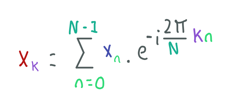
Fourier Transform Equation.

The idea behind this equation comes from the Fourier Series which tells us that we can use a sum of sine and cosine functions to represent a Periodic Function. Thus, the Xn term in the Fourier transform equation is this periodic function that we want to represent using sine and cosine functions.

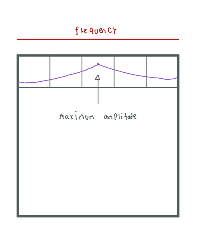
As we know, sine and cosine functions have amplitude, phase and frequency so we can build these functions using these properties.

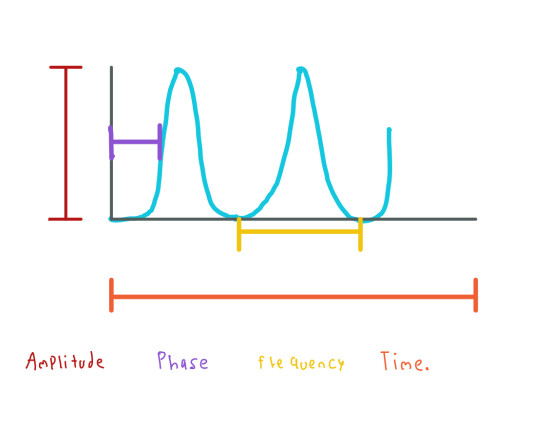
What the Fourier Transform do is decompose the periodic function into frequency, amplitud and phase values.

Here we say: the periodic function contains these amplitudes and phases at these frequencies. Thus, we can use these elements to build cosine and sine functions that together ensambled the original periodic function.

If we want to understand all the terms in the Fourier Transform equation we have to learn some math.

Complex Numbers

In the Fourier equation we can notice the term i, this term represents an imaginary number. In some equations we could have j instead of i, both represent the same. To understand what an imaginary number is let's check the following image:

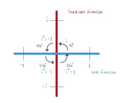
We can see an imaginary number as a rotation in the number line. When we see the term i this means a rotation of 90-degrees. Using two rotations of 90-degrees we go from 1 to -1 or from -1 to 1:

i ^ 2 = -1

i ^ 4 = 1

i ^ 6 = -1

i ^ 8 = 1

When we put an imaginary number and a real number together we form a complex number:

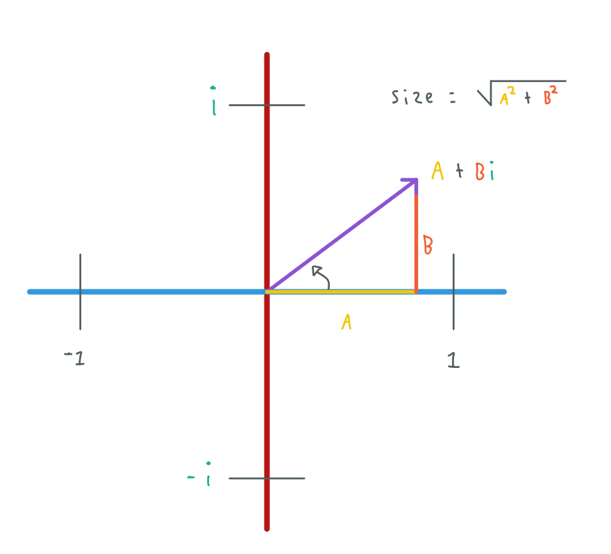
A is the "real" part or number and B is the imaginary part.

We can plot a complex number as a vector using the real an imaginary dimensions, we can also measure (get the size of a complex number) a complex number using the pytagoras theorem just as implied in the previous image.

Complex numbers are pretty useful, for example, let's imagine that we have a vector represented by the complex number 4 + 3i and we want to rotate this vector 45-degrees:

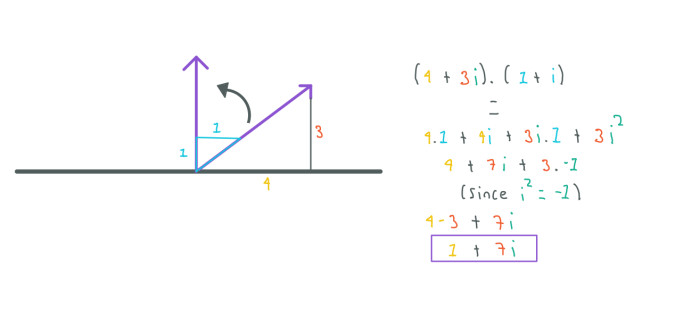
Using complex numbers we can just multiply our complex number by:

1 + i

Here B is 1 so we don't write it.

to rotate the vector. To understand why we used the complex number 1 + i we have to transform from cartesian to polar coordinates:

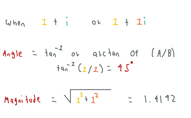
Polar coordinates are written in terms of magnitude and angle of the vector, in this case we only computed the angle using the inverse tangent function. As we can see the vector 1 + i has an angle of 45-degrees. Thus, when we multiply our complex number by 1 + i we rotate the complex number 45-degrees.

Complex numbers can also be negative or only have the imaginary part:

A - Bi

0 + Bi or just Bi

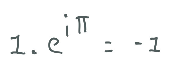
Euler's Formula

The equation for the Euler's Formula is the following one:

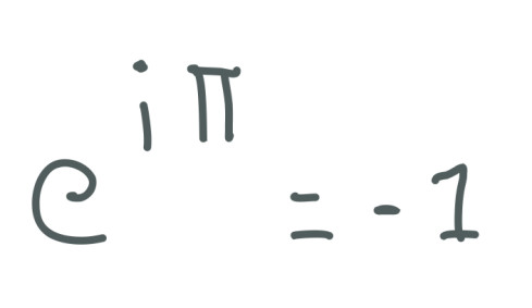
As we can notice, this equation contains an imaginary number in terms of radians. The result of this equation is -1, we have to remember that:

PI radians = 180-degree

2PI radians = 360-degree

What this equation describes is circular motion, if we start in 1 and we multiply by the Euler's Formula we end in -1:

We can also rewrite the equation using the cosine and sine functions:

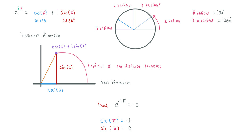
In the example above is more clear that using e we want to express a rotation which distance is given by PI or X in radians.

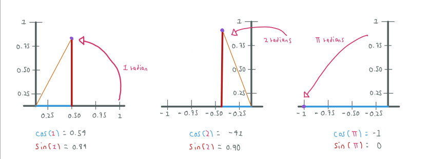
We can notice how by increasing the radians from 1 to PI radians we move from 1 to -1.

When we use the euler number e with a real exponent this means growing along the real axis whereas when we use an imaginary exponent, like in the Euler Formula, this means rotation around the imaginary axis.

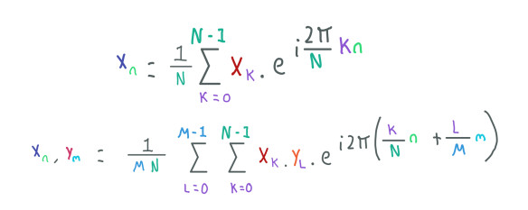
The Fourier Transform equation

The Euler Formula that we have just seen appears in the Fourier equation. In this case we have -i 2 PI Kn, since we are using 2 PI radians the rotation is around the whole circle and not just the half, also we have a negative term which means the rotation is clockwise. The term Kn is a specific frequency at which the rotation occurs.

Previously I had mentioned that Xn is the periodic function that we want to decompose, this partly true. To use the Fourier Transform we have to sample data from the periodic function. Hence, Xn is the n sample from the periodic function X and N is the number of samples that we obtained.

To decompose the periodic function we test many frequencies Kn, for each frequency that we test we use all the N samples Xn from the periodic function.

As we saw, the Euler Formula can be written using cosine and sine functions. As we rotate around the circle, what we are doing is building a sinusoid function (made of cosine and sine functions) at a specific frequency Kn. Since we are multiplying Xn with the Euler Formula, these circles will vary in size.

We use the Euler's Forumula in the Fourier equation due to its simplicity. Using the cosine and sine functions would complicate the equation.

The original periodic function X can be composed of one or multiple frequencies. If we are using a frequency Kn which X is composed of, the sinusoid function will match X.

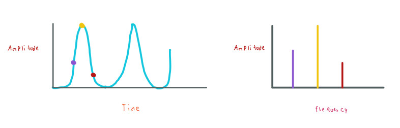
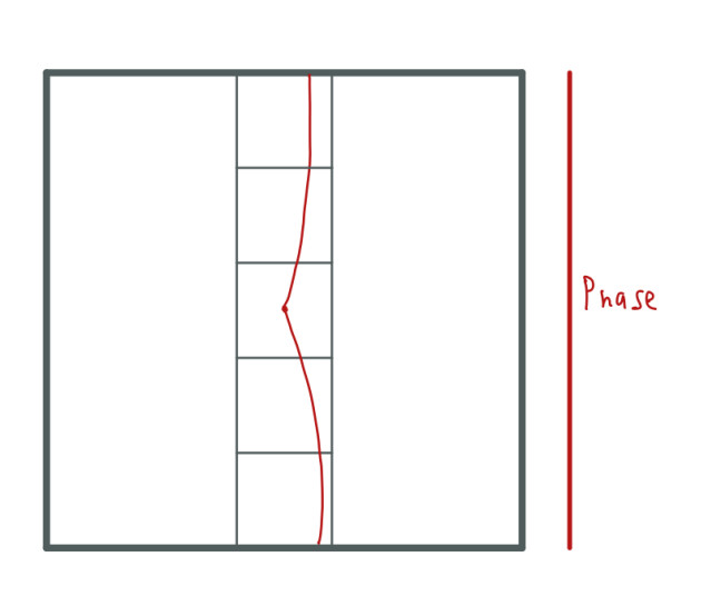
The Fourier Transform returns one complex number for each tested frequency so the complex number and the frequency are related. When we have a periodic function composed of multiple sinusoid functions at different frequencies and we match one of those frequencies, the complex number related to that frequency contains the amplitude and phase values to recreate one of the sinusoid functions. Computing the magnitude of the complex number we obtain the amplitude and computing the angle we obtain the phase. To further understand this let's see an example:

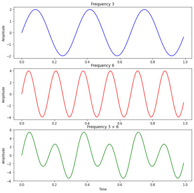
Here we have three periodic functions with different amplitudes, the first function has a frequency of 3, the second a frequency of 6 and the third function is the sum of the first two functions, thus, is composed of two frequencies, 3 and 6.

If we use the Fourier transform in these three functions and plot the amplitude at each frequency we obtain the following image:

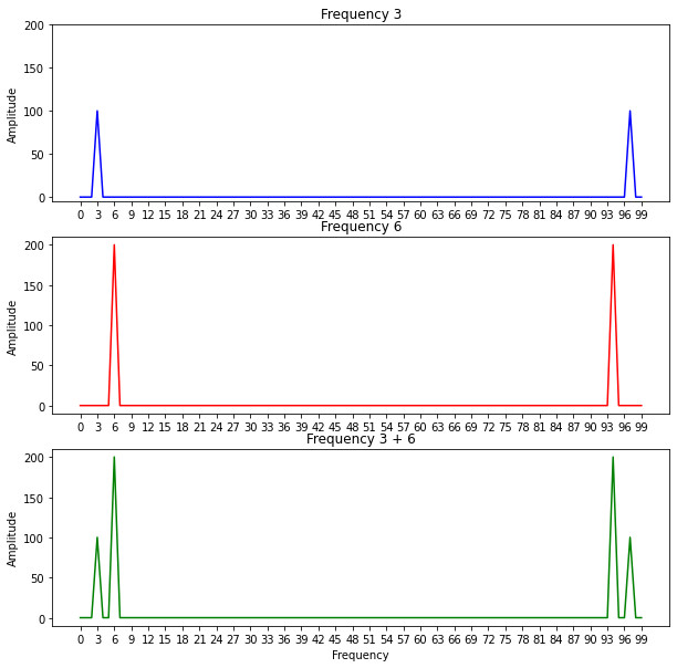
We can notice that the amplitude values increase as we aproach the correct frequencies. Since the third function is composed of two functions with different amplitudes and frequencies this is reflected in the plot.

However, we can also notice that the values at the end of each plot are repeated and the amplitude values are not correct. We can get rid of the second half of the frequency values since they are only a mirror version of the first half and normalize all the values to get the correct amplitudes:

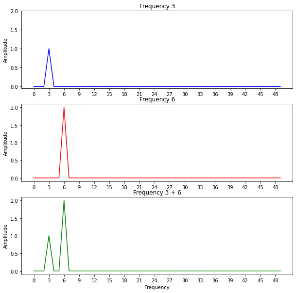
Now that we have a better example we can appreciate that we can get the same transformation of the third function if we sum the first two transformations. Thus, we could use the Fourier Transform before or after we compose a function and get the same result if we add up the transformed parts.

The aspects behind the Fourier Transform can be hard to understand without animations or gifs so here are some good videos to further understand the concepts:

Discrete Fourier Transform and Inverse Fourier Transform

The Fourier Transform can be used with images and the idea remain the same. We can decompose an image into multiple frequencies, thus, images are made of multiple frequencies. In fact the Fourier Transform that we have seen so far is called the Discrete Fourier Transform and as its name suggests is used when we have discrete data like pixels in images.

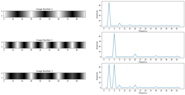
The image number 3 is composed of the first two images. When we use the Fourier Transform we get the frequencies which the images are made of. Our first two images are quite simple so they are only made of one frequency, the image number 3 is made of the two frequencies of the first images. We can notice that these are the same frequencies that we got with the periodic functions in the previous section.

Here the amplitude is given by the intensity of each pixel and since the pixels values are the same for all the images also the amplitude. We usually don't plot the 0 frequency since it contains the average of all the pixels.

In numpy, and multiple other libraries or frameworks, we use a function called Fast Fourier Transform that computes the transformation faster only lossing a little bit of accuracy.

In the case of images, if we have N pixels, we will test N frequencies from 0 to N-1. Let's use the first image and obtain the complex number that correspond to the frequency value of 3:

Using the Fast Transform from Numpy:

transform_1.shape # 90 Image width = 90

transform_1[3] # 4118.54089354984 + 8.526512829121202e-14j complex number from the 3 frequency

abs(transform_1[3]) # 4118.54089354984

When we use the function abs from Python or other libraries with a complex number this function computes the magnitude of the complex number.

Using the Discrete Transform manually:

def fourier(xn, Kn, current_n_index, N):

  pi_cicle = (-2 * math.pi) / N

  cicle = pi_cicle * Kn * current_n_index

  value = xn * np.exp(np.complex(0, cicle))



  return value

Kn = 3

N = len(simple_image[0])

arr = []



for current_n_index, xn in enumerate(simple_image[0]):

  complex_number = fourier(xn, Kn, current_n_index, N)

  arr.append(complex_number)

current_f = np.sum(arr)

current_f # 4118.540893549842-2.0463630789890885e-12j

abs(current_f) # 4118.540893549842

Here we can notice that the imaginary part of both results is different but since its a really small number this doesn't affect the final result, the magnitude of both numbers is the same.

In numpy we can create complex numbers using the np.complex function, in the previuos example we created a complex number only with the imaginary part that corresponds to the Euler's Formula.

Let's also compute a tiny part of the Fourier Transform in paper using the frequency value 4 and the sample number 5:

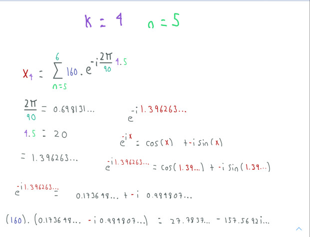
We have to remember that the exponent is negative but thanks to the properties of cosine and sine functions we can use this exponent outside the functions:

cos(-x) == cos(x)

sin(-x) == -sin(x)



Thus:



cos(-x) + isin(-x) == cos(x) - isin(x)

We can corroborate these computations in code:

The original complex number

arr[5] # (27.783708426708866-157.56924048195327j)

len(simple_image[0]) # 90

simple_image[0][5] # 160

In numpy we use j instead of i.

(2 * math.pi) / 90 # 0.06981317007977318

0.06981317007977318 * 20 # 1.3962634015954636

np.cos(1.3962634015954636) # 0.17364817766693041

np.sin(1.3962634015954636) # 0.984807753012208



(160 * 0.17364817766693041) # 27.783708426708866

(160 * 0.984807753012208) * -1j # -157.56924048195327j

We can also directly create a complex number and get the same result:

160 * np.exp(np.complex(0, -1.3962634015954636)) # 27.783708426708866-157.56924048195327j

You can find all the code in the same Jupiter Notebook.

To compute all the Fourier Transforms that we have seen, we have used 1D data, in the case of the images we only used the first row of each image. This is called 1D Fourier Transform along the x-axis. However, images are 2 dimensional so we need a Fourier Transform along y-axis as well, in other words, we need a 2D Fourier Transform:

Now we have N pixels along the x axis and M pixels along the y-axis.

The 2D Fourier Transform of an image is an array of the same size where each cell contains a complex number. As we know if we compute the magnitude of a complex number we obtain the amplitude. We can plot these amplitudes, however, we need to scale them so we can visualize them correctly. This scaled version is called the image's spectrum:

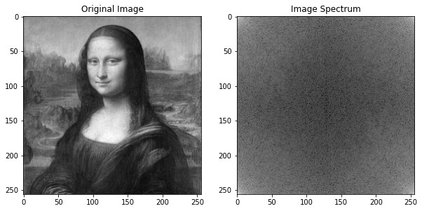
img = cv2.imread("real_image.jpg", 0)

transform_2d = np.fft.fft2(img)

spectrum = np.log( 1 + np.abs(transform_2d))

Using numpy to compute the 2D Fourier Tranform and to scale the magnitudes.

We could also plot the phase of the image computing the angle of the complex numbers but this is not usually done.

Something that we often do is put all the low frequencies in the center of the spectrum and the high frequencies in the sorruoundings:

centered = np.fft.fftshift(transform_2d)

centered_spectrum = np.log( 1 + np.abs(centered))

This is a frequent task that numpy already has a function (np.fftfftshift) to sort the frequencies. This new way of presenting the frequencies is quite useful to preprocess the image and apply filters.

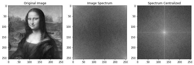
In an image, low frequencies represent pixels that change slowly so we have the most part of the image information in low frequencies whereas high frequencies represent pixels that change dramatically like borders or edges. We can use filters to remove the low or high frequencies of an image. Since all the low frequencies are now in the center of the spectrum is really easy to apply these filters:

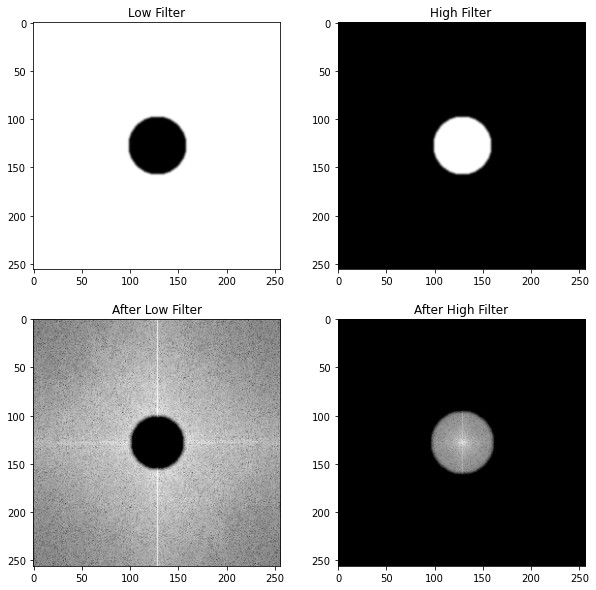
low_filter_center_transform = centered * low_filter

high_filter_center_transform = centered * high_filter

We have to use these filters and all the computations we want in the centered image and not in the centered_spectrum image, this image is only used to visualize the amplitudes correctly.

Now that we have removed low or high frequencies we have to move back the frequencies to their original position. In numpy we can use the following function to get this done:

low_filter_transform = np.fft.ifftshift(low_filter_center_transform)

high_filter_transform = np.fft.ifftshift(high_filter_center_transform)

We have our preproccesed images in the frequency domain. What we want is to transform back the images to the time domain to see how the filters affected the image. Due to this necessity we have the Inverse Fourier Transform:

1D and 2D Inverse Fourier Transform.

This transformation takes the image in the frequency domain (Xk, YL) and returns the image in the time domain (Xn, Ym) in form of complex numbers but this time when we compute the magnitude of these complex numbers we have the pixels values back.

In numpy we can use the following function to compute the 2D Inverse Fourier Transform:

origina_low_filter = np.fft.ifft2(low_filter_transform)

origina_high_filter = np.fft.ifft2(high_filter_transform)

Thus, now we can see the result of applying the low and high frequency filters:

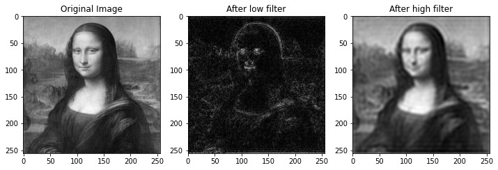
We can notice how after the Low Frequency Filter we got back the border and edges of the original image and after the High Frequency Filter we got back most part of the information of the image but without the High Frequencies that give a sharp aspect to the image.

We can also take advantage of this transformation in other ways. For example, convolution in the spatial/time domain is multiplication in the frequency domain. Hence, we could save time and computations using the frequency domain to apply convolutions.

MRI

Our body is made of billions of atoms, most of these are hydrogen (H) atoms since our body is composed of 60 of water. The hydrogen nucleus consists of one single proton. These protons and the whole nuclei have an interesting quantum property called Spin Angular Momentum which makes protons behave as if they are spinning, although they are not really moving, also these nuclei have a second property called Magnetic Moment that makes the proton behave like a magnet. Hydrogen is the most used atom in MRI but is not the only one that we can use.

Before move on, we can notice that in MRI we can use the terms protons, nucleus, and spins interchangeable. So, from now on we will use the term spin to refer to the proton inside the hydrogen nucleus.

Atoms have a property called Gyromagnetic Ratio (Y) which value varies from atom to atom. This property is related to the Magnetic Moment of the spin.

In MRI we use a lot of Magnetic Fields to change the behavior of the spins. When we put the spins in a magnetic field, these will try to align with this magnetic field, some will align in the same direction and some others in the opposite direction.

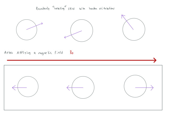
We can make an average of all these spins to create a big vector called Net Magnetic Field or M. Since most of the spins are pointing in the opposite direction, M will point to that direction as well. Having M makes the work easier since we can use classic physics to measure and understand our spins, that's why we can represent M as a vector.

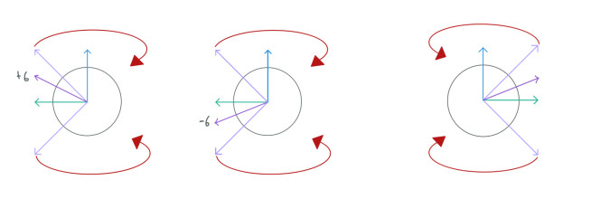
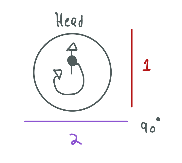
However, since our spins are "moving" the magnetic field will give the spins a different motion that we call precession. Hence, the spins will be rotating or precessing randomly but pointing to the direction of its magnetic moment. In the following image the dark purple arrow indicates the direction of the spin and the lighter purple arrows indicate the angles that the dark arrow can rotate around.

To have a better understanding of this, it's a good idea to imagine a Gyroscope. Similarly to spins, gyroscopes also have a property called angular momentum. The gyroscope will start moving when we apply a force. But since the gyroscope is being affected by the gravity, the gyroscope will rotate or precess.

The magnetic field that we use is known as the main magnetic field or B0. In some texts, I have found that the spins are in reality always precessing due to the magnetic fields of the earth and B0 only sustains this precession. However, it's easier to understand if we say that the spins precess due to B0, hence, let's ignore this.

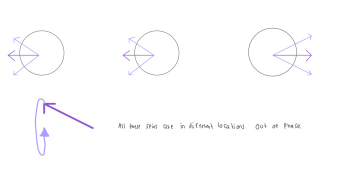
Given that the spins are precessing in random orientations when we take the average of these spins to make M the spins cancel each other out. We can see this more clearly in the next image.

This could be hard to understand but the idea is that we remain only with longitudinal components of each spin vector. These longitudinal components cancel each other out as well. However, we usually have more longitudinal components pointing in the opposite direction, thus, when we take the average of the spins the final vector M will point in that direction:

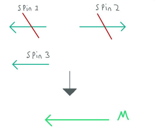
Since we remain only with the longitudinal components M will not precess. Despite this, all the spins are still precessing all the time. The dephase of these spins vanish their transversal components. This dephase is caused by the random orientations of each spin.

B0 is not the only magnetic field used in the MRI machine, we have another one called B1. This magnetic field is used to change the energy of the spins. When the spins have a change in their energy some of them will be in phase aligned. Thus, their transversal components won't cancel each other out and they will generate transversal magnetization. This magnetization makes M to start precessing which generates a signal called MR Signal.

We can see this as a 90-degree "rotation" of the spins so their longitudinal components change place with the transversal components. Hence, the longitudinal components loss signal and the transversal components gain signal.

Now, to get this done we have to remember the property of the atoms called Gyromagnetic Ratio (Y), when we apply the main magnetic field B0 the spins begin to precess at a specific frequency called Larmor Frequency. The value of this frequency is given by the following formula:

W0 = YB0

Where W0 is the final frequency, Y is the Gyromagnetic Ratio and B0 is the strength of the main magnetic field. To create a change in energy and put in phase the spins, B1 has to produce a radio frequency wave in the same frequency (W0) at which the spins are precessing, this is called resonance.

B1 must be orthogonal to B0 (90 degrees). Usually B0 is in the Z-axis of the MRI machine.

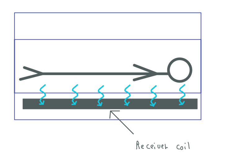
Until now we have seen two magnetic fields B0 and B1. These two magnetic fields are produced by coils. B1 uses RF Coils which can transmit or receive radio frequency waves. When we use B1 to start precessing M, the latter generates an MR Signal that is captured by a receiver coil.

Here put the coil along with the machine and the body.

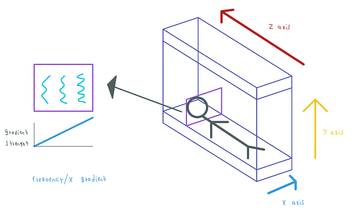
Gradient Coils

As we have seen the net magnetic field M when processing produces an MR signal, this signal is composed of all the tiny signals from billions of spins. Even when we have billions of spins precessing, only a part of them generates signals. These spins are the ones that are in phase after B1 is used.

The spins' signals that compose the MR signal comes from all the parts of the body, from the feet to the head. So we don't really know where the signal comes from. To localize the signal we use a special set of coils called Gradient Coils.

These gradient coils also apply magnetic fields which affect the main magnetic field B0.

Slice Gradient

This gradient is applied along the Z-axis. The strength of this gradient increases linearly which makes B0 to also change its strength from bottom to top:

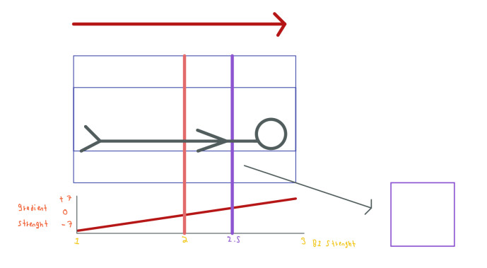
The red line indicates how the gradient coil Z is applied, in the left we reduce the strength of the magnetic field B0 and in the right we increase its strength. The pink line indicates the center of the machine where the strength of B0 is the same as the original since the strength of the coil gradient Z is 0 in this position.

The variation in strength along the main magnetic field B0 will make the spins precess at different frequencies:

W0 = YB0

W0 = Y(1.5)

W0 = Y(2.5)

W0 = Y(2.9)

And as we can remember, B1 needs to use the same frequency as the spins to transmit the energy efficiently. For instance, if we put B1 at a frequency:

W0 = Y(2.5)

Only the spins that are precessing at the same frequency will receive the energy correctly and thus generate a signal. This is showed in the purple line in the previous image, where only the spins in this slice will rotate after B1 is used at the W0 = Y(2.5) frequency. If we want signals from a different area of the body we can change the frequency of B1 and match the frequency at which the spins are precessing in the desired area.

The Z gradient is also called the slice gradient for this reason. We use this gradient at the same time that we apply B1.

Frequency Gradient

Currently we have an MR signal that comes from a whole slice but we don't how much signal comes from each point in that slice. To overcome this, we will use two more gradients in the X and Y axes. The first gradient is called the frequency encoding gradient and is usually applied in the X direction:

This gradient is used in a similar way than the slice gradient. As we will further see, we need to sample the MR Signal to obtain information from the spins. The frequency gradient is used to change the strength of B0 inside the slice that we previously obtained. Hence, the spins inside the slice will precess at different frequencies and their signals will have the same frequencies then we can localize these signals along the x-axis by their frequencies values.

Phase Gradient

By now we have an MR signal that comes from a slice and we can detect the signals from the spins that compose the MR signal along the x-axis. However, we don't know yet how much signal comes from the y-axis. We can use one more gradient in the y-direction to create differences in the phase of the spins. This gradient called phase gradient is somehow harder to understand.

So far we have seen the following steps:

1. We apply B1 and the slice gradient at the same time.

2. We turn off these two coils.

3. After some time, we sample the MR signal that comes from M at time TE, we will see more about this in the next section, and we turn on the frequency gradient.

To dephase the spins we have to use the phase gradient between the 2 and 3 steps. This gradient will "stop" the spins for some time, once we have turned off the gradient, the spins will have a dephase. When we sample the MR signal, all the information is saved in an array called the k-space.

When we use the frequency gradient and sample the MR Signal the information is saved in the columns of the k-space. Unlike the frequency gradient, we have to repeat all these steps for each row that we want to fill in the k-space. These rows will have a difference in the phase that makes them differentiable. We will see more about the k-space in further sections.

We have learned that the signals from all the spins are averaged in the net magnetization field M. Using the slice gradient we make that only the spins from some area in the body contribute to form M. Furthermore, using the phase gradient these spins will have some dephase, and using the frequency gradient our final MR signal will be composed of multiple waves of different frequencies and phases. The receiver coil detects this composed MR signal.

T2, T1 decay.

The MR signal contains all the information that we need to create the MRI Image. We can get this information sampling the MR signal.

First, we have to know that the MR signal decays over time. We call this the Free Induction Decay. After some time the MR signal, which is generated by the transversal magnetization of M, decays until all the signal is lost.

The spins that underwent the 90-degree "rotation" eventually return to their original position where they have longitudinal magnetization but no transversal magnetization. Hence, the spins lose transversal magnetization, an effect that we call T2, and gain or recover their longitudinal magnetization, an effect that we call T1.

The Free Induction Decay is relevant since different kinds of tissues lose transversal magnetization and gain longitudinal magnetization at different rates due to their atomic configuration of hydrogen. For instance, tissues with fat areas lose transversal magnetization faster than areas with fluids like the cerebrospinal fluid.

This contrast between tissues is useful when we want to assign different intensities or colors to the pixels of the MRI image. If the tissue's signal decays fastly their corresponding pixels/voxels in the MRI image will have a dark or gray color whereas if the tissue's signal decays slowly their corresponding pixels/voxels in the MRI image will have a brighter or white color.

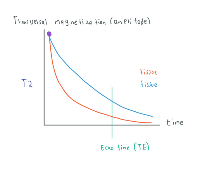
In the image above we have the signal decay of two different tissues. We also have an Echo Time (TE) represented by a green line. The value of this echo time is chosen by us and indicates the time when we start sampling the signal.

To obtain a useful and high-quality image, we have to choose a good echo time where the contrast between tissues is clear.

In the previous image, we can notice that the signals from both tissues start in the same purple point. However, this is not always the case, this signal also depends on the proton density of each tissue:

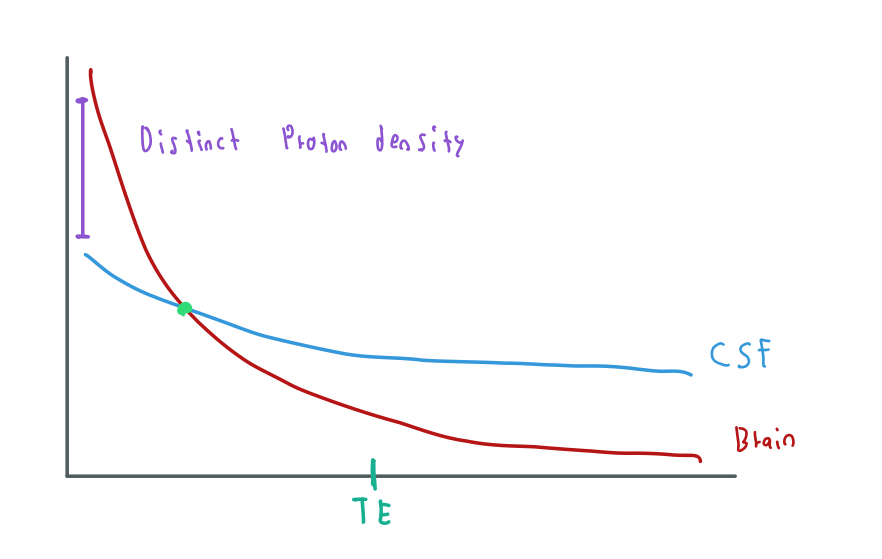
This complicates the sampling task because now we have to be aware of the time to obtain the contrast that we want. For example, now we have a green point where both tissues' signals have the same amplitude, thus, they will look the same in the final image if we sample at this time.

Additionally we have one more problem. As we have seen the frequency at which the spins precess is given by the Gyromagnetic ratio and the strength of B0. However, we have to take into account magnetic variations found in tissues and the main magnetic field B0. These small variations affect the behavior of the spins. We call this Magnetic Susceptibility.

Due to this Magnetic Susceptibility, more spins are dephased and precessing at diverse frequencies in different tissues.

W0 = Y(B0 + X)

Where X are the variabilities in tissues and Magnetic Field.

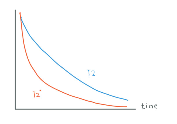
The orange line shows a more realistic T2 that takes into account the variabilities in magnetization. This T2 decays faster so it's harder to sample the signal.

As mentioned earlier, B1 transmits energy to the spins which makes them be in phase with each other so we can obtain transversal magnetization, hence, a signal. The variabilities in magnetization cause a loss in the phase of the spins something that eventually makes them cancel each other out. This is why the signal decays faster.

To solve this we can use B1 again to give more energy to the spins. Currently, we use B1 for a short time to generate a 90-degree "rotation" and then we turn it off. We can leave B1 for a longer time to generate a 180-degree "rotation". This new transfer of energy will make the spins be in phase after a period of time so we can recover the signal. This technique is called Spin Echo.

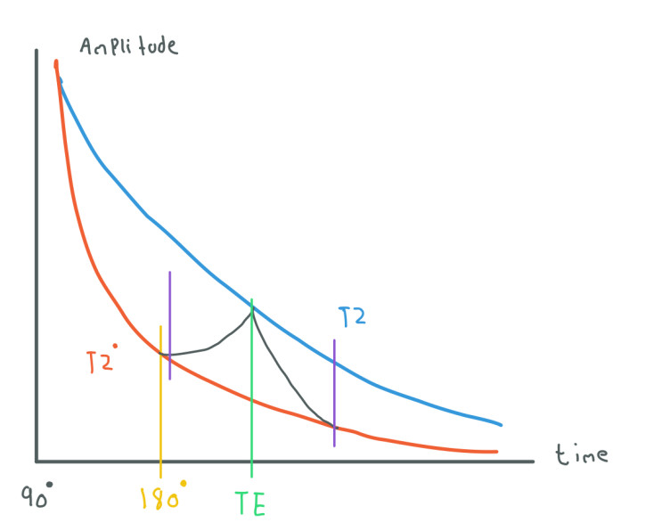
We can see how after we use the 180 pulse the signal starts recovering amplitude. However, this signal will decay again so we want to sample it when the signal reaches its maximum amplitude (TE). T2 can't be directly measured, it is just an ideal state of the signal. We can use the 180 pulse whenever we want as long as we still have a signal.

In this example, we can also notice that we have two purple lines. These lines indicate the start and the end of the sampling of the signal. The sampling task takes some time to be ready so we want to start a little bit before the echo time (TE). This sampling is important as we can observe that the amplitude increases and then decreases. This change will be reflected in the k-space.

Having seen T2 let's check how T1 works:

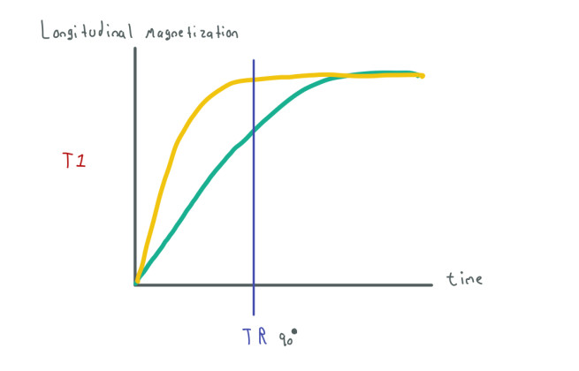
In this case, spins are recovering their longitudinal magnetization. This process usually occurs slower than T2 and is also different for each kind of tissue. If fluids in T2 lose their transversal magnetization fastly, in T1 fluids recover their longitudinal magnetization slowly. We can use T2, T1, or take both into account to assign colors to the pixels in the MRI image.

In the case of T1, we have a variable called repetition time (TR) which value is chosen by us. This repetition time indicates the time when we can use another 90-degree pulse (B1) to give energy to the spins and get another signal.

This new 90-degree pulse is used after the Spin Echo. A combination of all pulses (B1) and sampling times can give us different kinds of MRI images.

K-Space

Now that we have learned about the MR signal and the several coils used to modify this signal we can start talking about the k-space.

The k-space is a tensor or array where we put the information that we obtain from the MR Signal. This space is similar to the space that we get when we use the Fourier transform in an image. Hence, this space contains amplitudes and phases from the signal in each cell as a complex number.

By now we have seen the following steps:

• We use B1 to "rotate" the spins that are precessing in B0 along with the slice gradient to only give energy to some specific spins.

• We turn off B1 and the slice gradient.

• The signal begin to decay.

• We turn on the phase gradient to "stop" the precession of the spins and create some dephase.

• We turn off the phase gradient.

• We use an Spin Echo to recover the signal and we start sampling (Echo Time), at the same time we turn on the frequency gradient.

To sample the MR Signal we have to transform the continuous signal into a discrete signal (digitalize the signal). This is done by a device called A2D. This device will sample the signal multiple times and save the information of amplitude and phase at each sample time. Sometimes MRI machines use two coils to receive information from the MR Signal. These two coils are orthogonal to each other (90-degree variation) which makes them receive different information from the MR Signal. When we use two coils is easier to split the information into real and imaginary parts to form the complex number that is saved in each cell of the k-space.

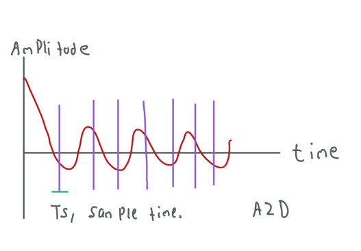
Each purple line represents a sampling time.

This MR signal has been already altered by the phase and frequency gradients. Therefore, now it contains information from multiple signals at different frequencies and phases. We can save this information in the first row of the k-space:

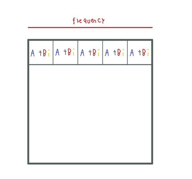
Each cell contains information about the amplitude and phase sampled from the MR signal in the form of a complex number.

As an example we could say that: In the first cell we have the amplitude and phase from a signal which frequency was X. For this reason, we used the frequency gradient so we can localize information with respect to its frequency.

To get information for one more row we have to repeat all the past steps but using a different strength for the phase gradient. Hence, the information between rows will have a contrast in phase and the information between columns will have a contrast in frequency.

For instance, if we want an MRI Image slice of size 512x512 we have to repeat this process 512 times and sample the signal also 512 times. Sampling the signal is not computationally expensive but repeat all these steps multiple times does take time.

As we can remember, when we use the Echo Spin the MR signal recovers its signal and then decays again. We sample the signal as this change occurs, something that is reflected in the information that we save in the k-space:

Thus, the first half of the cells of each row contain amplitudes that increase their value and the other half of the cells contain amplitudes that decrease their value, reaching a peak in the center of the row.

This also occurs as we approach the center of the k-space in the y-axis. The phase gradient strength is bigger as we move out from the center and smaller as we advance the center:

Since the gradient strength is bigger as we move out from the center, the dephase of the spins is greater what leads to loss more signal in these areas. The signal loss leads to a smaller or bigger amplitude.

Furthermore, the frequency of the spins is given by:

W0 = Y(B0 + x) 

When we apply the phase and frequency gradients this alters the strength of B0, thus, the frequency of the spins. As we said, in the center of the k-space we have the smaller strength for the phase and frequency gradients then the frequency in this area is low, as we move out from the center, the frequency is higher due to bigger strength in these gradients.

In summary, in the center we have the bigger amplitudes and the lower frequencies and as we move out from the center we have smaller amplitudes and higher frequencies.

When we plot the k-space we usually see a white area in the center of the image, this is due to the bigger amplitudes values living here.

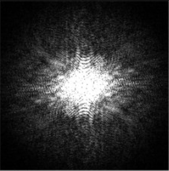
Original image from www.researchgate.net

High-frequency components contain information about the corners and edges of the MRI image and low-frequency components contain information about the appearance of the image.

Each cell in the k-space represents spatial frequencies and not correspond one-to-one to the cells or pixels in the MRI image.

To get the MRI image we apply the inverse Fourier Transform to the k-space. Of course there are some preprocessing steps used to obtain a higher quality image.

To finish this section there is one more important fact about the k-space. In the k-space exists symmetry between rows and columns:

The yellow and orange points have the same values even when they are in opposite cells.

Due to this symmetry, we could also only get information to fill half of the k-space and estimate the other half and don't lose too much information.

This technique is called Partial Fourier Imaging.

We can do this from left to right or from top to bottom. If we do this from top to bottom the process is faster since we need to compute fewer rows.

Accelerated Parallel Imaging

In this section we will learn about a technique that is highly related to the problems that the paper is trying to solve.

During the MRI process we use a receiver coil to detect the MR signal produced by M. In the previous section I mentioned that we can use two coils to detect the MR Signal and get more information.

As the spins precess the signal is generated and is received in both coils. When the spins are parallel to one coil, this coil does not receive the signal but the other coil does.

We can use two orthogonal coils like the ones in the example above to obtain more information from the MR signal and get the real and imaginary components that we save in the k-space more easily. The signals from both coils are combined and stored in one k-space array. However we can opt to not combine this information and instead create two k-space arrays.

Here we have two coils at two sides of the head. If we repeat all the steps that we have seen we can fill two k-space arrays at the same time using these two coils. Each coil is more sensitive to the area near the coil. Therefore, the signal is better when the tissue that produces this signal is near the coil.

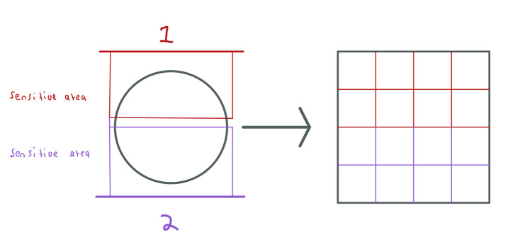
The first coil can collect information from the first half of the head and the second coil can collect information from the other half of the head. Thus, we could just only sample 256 rows to generate an MRI image of size 512 using the k-space arrays from both coils and obtain an image with good quality.

We can use several more coils, each will be sensitive to some area in the body. With this knowledge, we can combine the k-spaces from all the coils to produce an MRI image faster.

When we fill the full k-space arrays the technique is called Parallel Imaging whereas when we only fill a part or undersampled the k-space the technique is called Accelerated Parallel Imaging.

In the previous example, we undersampled the k-space and combined both k-space arrays to create the MRI image.

We can see an example of sensitivity maps in figure 2 of the fastMRI: An Open Dataset and Benchmarks for Accelerated MRI paper.

Classic Approaches.

To get an MRI image from multiple undersampled k-space arrays there are two popular techniques, SENSE and GRAPPA.

SENSE is quite easy to understand, the idea is to combine reconstructed images from undersampled k-space arrays. Thus, we first reconstruct the images from the k-space, even if this space is not complete, using the Fourier Transform and then we combine the images.

Let's imagine that we have nc coils, since we are using only a part of the k-space, each reconstructed image i of nc images will contain overlapping frequencies because we are sampling fewer frequencies. Hence, the reconstructed image will look fold-over.

For example, if we sampling every two frequencies, the information from all the spins will be still in the k-space but each row or column will contain information from two signals (aliasing).

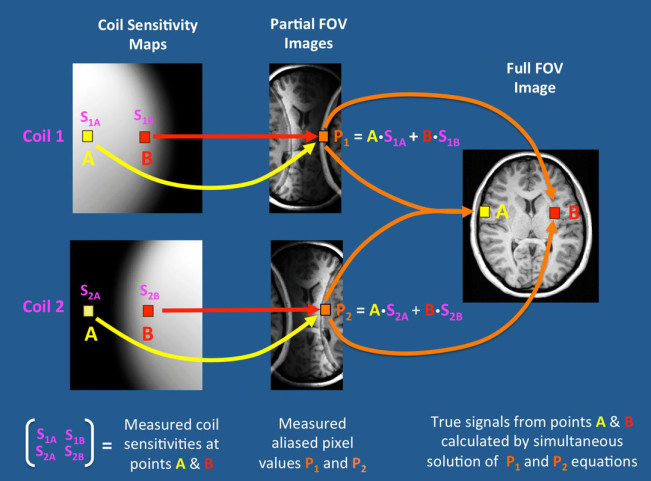
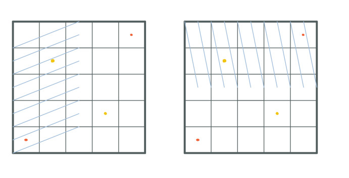
This image from http://mriquestions.com/ explains really good this process. The Partial FOV Images are the reconstructed images from two undersampled k-space arrays. We can notice that all the information is there but overlapped.

In this example we have an MRI signal that arises from the point A, the two coils have different sensitivity to that point S1A and S2A. Due to the overlapping, the points A and B end up in the positions of the same pixels P1 and P2 in each image. Thus, each pixel is composed of two signals. We want to know how much signal belongs to the points A and B to unfold the image. We can achieve this with the help of the sensitivity maps and solving two equations:

P1 = A.S1A + B.S1B

P2 = A.S2A + B.S2B

You can check the http://mriquestions.com/ page for more information about these techniques or about MRI in general.

In the case of GRAPPA what we want to do is fill the missing values of the k-space before the reconstruction of the image.

Something that is stated in this technique is the fact that the lines in the center of the k-space are fully sampled. As we learned, in the center of the k-space are the low frequencies that compose the most part of the image. Furthermore, the sensitivity maps usually are computed from the center of the k-space.

The estimation of the missing values of the k-space is a complex process that is not especially important now since we are going to solve this using neural networks.

Once we have the k-space filled, we use the Fourier Transform to generate nc images from nc coils. To obtain the MRI image we have to combine these nc images using the root sum of squares:

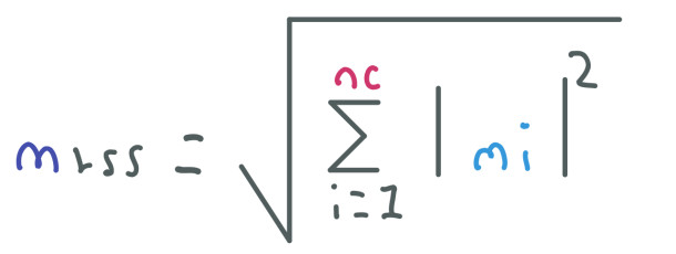
This method is also used in both papers as we will further see.

The undersampling direction of the k-space is always the direction of the phase gradient to reduce the time. As we know, the phase and frequency gradients can be applied horizontally or vertically.

Deep Learning Techniques

In the paper fastMRI: An Open Dataset and Benchmarks for Accelerated MRI the authors suggest one procedure to reconstruct an image from multiple undersampled k-space arrays using deep neural networks:

1. Having a set of undersampled k-space arrays we can fill the missing data with zeros.

2. Apply an Inverse Fourier Transform to the zero-filled arrays to get overlapped images.

3. Compute the absolute value of the overlapped images.

4. Combine the images using the root sum of squares.

We can use an architecture like the U-net model and feed the combined image as input. We can notice that this procedure is similar to SENSE where first we reconstruct the image and then we fix it.

In the same paper the authors introduced a dataset that includes four types of data:

1. Raw multi-coil data, the same that we get from the coils to fill the k-space.

2. Emulated single-coil data. We won't use this type of data.

3. Ground-truth images reconstructed from fully-sampled multi-coils using the root sum of squares.

4. DICOM images with higher quality.

We don't have to confuse the kind of data. In medical images like MRI we usually have images of three dimensions where the last dimension is depth. From a 3d image we can get a 2d image which we call slice image. The Raw multi-coil data is data from multiple nc coils that we can combine to get one slice not the whole 3d image.

We can apply a mask to the raw multi-coil data to remove some columns or rows and simulate undersampled k-space arrays:

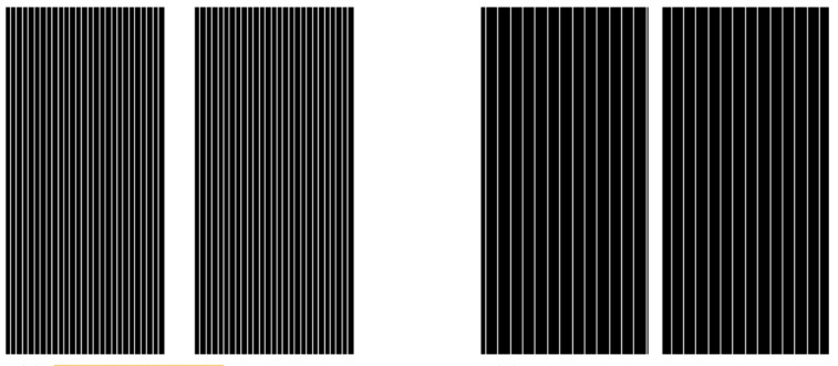
Image from paper fastMRI: An Open Dataset and Benchmarks for Accelerated MRI

On the left we have a mask that removes every 4 columns and on the right a mask that removes every 8 columns. We can notice how the columns in the center are not removed.

We then combine the masked nc images from multiple sets and use the reconstructed images as the input of the U-net model. Furthermore, we use the Ground-truth images, which are already reconstructed from fully-sampled k-space arrays, as labels.

We can use the mean absolute error L1 loss to train the U-net model.

Artifacts and Banding.

In MRI we could encounter some anomalies in the final image that reduce the quality of the latter. These anomalies knew as Artifacts are due to several reasons like the motion of the patient at sampling time, magnetic susceptibilities, and tissue or technique related. In the Classic Approaches section, we saw one of these anomalies called Aliassing when the reconstructed image was overlapped due to the accelerated parallel imaging technique.

When we use Deep Learning Approaches to reconstruct MRI images we can also encounter artifacts.

Banding artifact.

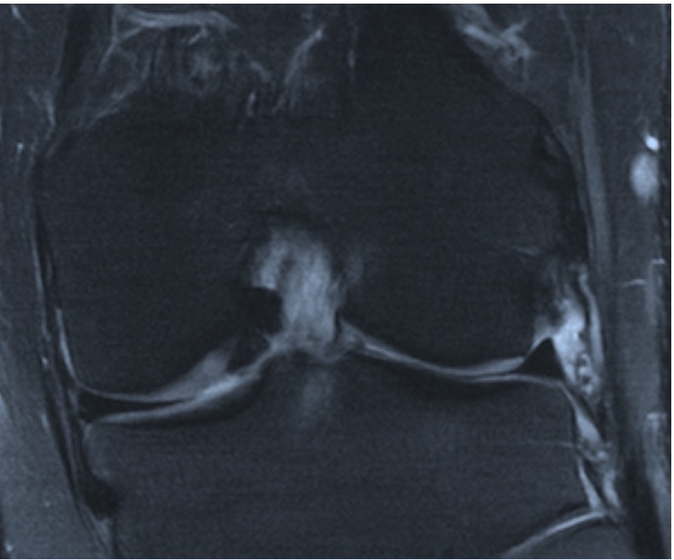
In fact, this is what the MRI Banding Removal via Adversarial Training paper is trying to solve. Here the Banding is an artifact produced by cartesian deep-learning reconstruction systems.

In the previous image we can notice this Banding horizontally. The Banding artifact has a streaking pattern exactly aligned with the phase encoding direction.

In this case, the authors used the k-space arrays (without reconstruction) masked every 4 columns as the model input, the output of the model is followed by an Inverse Fourier Transform and then the root sum of squares is used to get the final image. Additionally, the Ground-truth images are used as labels.

We can notice that this technique is similar to GRAPPA where first we fill the k-space and then we reconstruct the image.

To solve the banding problem the authors followed an Adversarial Training procedure that is quite simple but useful.

Firstly, the data in the fastMRI dataset (presented in the previous section) has a horizontal phase-encoding direction. However, we can change this direction sampling a random variable, if the variable is greater than 0.5 we transpose the k-space, thus, we change the banding direction. This is done before and after we feed the k-space to the model.

Knowing this, we can use a model that predicts the direction banding, which can be horizontal or vertical, from the final image. This model, which we call Adversary, is trained using the binary cross-entropy where the labels are the random variables that indicate if the k-space was rotated.

Now, what we want is to avoid the banding artifact. If the Adversary model is good predicting when the k-space was rotated then the banding is presented since this is the only hint of the orientation. On the other side, we train a Predictor model, this model generates the final image using the L1 and SSIM (Structural similarity) losses but with the banding problem. Thus, we add the inverse loss of the Adversary.

Therefore, the Predictor model has to fool the Adversary model generating a final image without the banding so the Adversary model won't be able to predict the orientation correctly. This is why is called Adversarial Training. This technique is the same that we use when we train GAN networks.

Training

The training consist of two phases, in the first phase we only train the Predictor model for 100 epochs where the adversarial loss is not included but we still rotate the k-space. Thus, the generating images manifest the banding artifact. In the second phase, we train the Predictor and the Adversary models for 60 epochs.

In this phase when the Predictor parameters are updated, the Adversary gradients are propagated to the Predictor but we don't update the Adversary parameters.

The training for the second phase in PyTorch looks like:

for epoch in range(epochs):

  for k_space, ground_truth in dataset:

    rotation_labels = ...

    k_space = rotate(k_space, rotation_labels)

    predictor_output = predictor(k_space) # returns filled k-space

    predictor_output = rotate(predictor_output, rotation_labels)

    reconstructed_images = reconstruct(predictor_output)



    # Predict Update



    for param in adversary.parameters():

      param.requires_grad = False # Still computes gradient with respect to predictor



    adversary_output = adversary(reconstructed_images)

    predictor_loss = compute_predictor_loss(reconstructed_images, ground_truth, adversary_output, rotation_labels)



    predictor_loss.backward()

    predictor_optimizer.step()

    predictor_optimizer.zero_grad()



    # Adversary Update



    for param in adversary.parameters():

      param.requires_grad = True



    adversary_output = adversary(reconstructed_images.detach())

    adversary_loss = compute_adversary_loss(adversary_output, rotation_labels)



    adversary_loss.backward()

    adversary_optimizer.step()

    adversary_optimizer.zero_grad()

Here we can notice the use of requires_grad and detach. In PyTorch when we compute the gradients using loss.backward(), we calculate the gradients for all the trainable parameters. Using requires_grad = False we avoid computing the gradients of the adversary model with respect to their own weights but we still compute the gradients of the predictor model with respect to the adversary model.

If we don't use requires_grad = False we can still train the model and update the weights without any problem since the optimizer:

predictor_optimizer = torch.optim.Adam(predictor.parameters(), lr=0.0003, momentum=0.9)

takes as input the weights/parameters that should be updated. However, we would compute unnecessary gradients of the adversary model which can be computationally expensive. Using detach() we have similar behavior, we avoid computing the gradients of the predictor that are not necessary when we update the adversarial model. In this case we also change back requires_grad to True so the adversarial gradients are estimated.

The training for the second phase in TensorFlow is the following one:

@tf.function

def train_step(k_space, ground_truth):

  with tf.GradientTape(persistent=True) as tape:

    rotation_labels = ...

    k_space = rotate(k_space, rotation_labels)

    predictor_output = predictor(k_space) # returns filled k-space

    predictor_output = rotate(predictor_output, rotation_labels)

    reconstructed_images = reconstruct(predictor_output)



    adversary_output = adversary(reconstructed_images)



    predictor_loss = compute_predictor_loss(reconstructed_images, ground_truth, adversary_output, rotation_labels)

    adversary_loss = compute_adversary_loss(adversary_output, rotation_labels)



  predictor_gradients = tape.gradient(predictor_loss, predictor.trainable_variables)



  adversary_gradients = tape.gradient(adversary_loss, adversary.trainable_variables)

Here we are using TensorFlow 2.0 that computes gradients using GradientTape. When we run code inside the GradientTape block, this block records all the operations which are subsequently used to estimate the gradients.

Unlike PyTorch, when we want to compute the gradients we use:

predictor_gradients = tape.gradient(predictor_loss, predictor.trainable_variables)

where we specify for what parameters the gradients are computed.

with respect to what parameters the gradients are computed?

where we specify what weights/parameters the gradients are computed for. Thus, we don't have to use functions like requires_grad or detach.

In the paper is stated that the training occurs simultaneously for both models in the same batch.

The Predictor model uses a sequence of 12 U-net models, the first U-Net takes as input the masked k-space which are complex tensors where we have real and imaginary parts. The output of the last U-net model is the reconstructed k-space tensor which we apply the inverse Fourier Transform and then the root sum of squares to obtain the reconstructed images.

The Adversarial model uses a shallow ResNet architecture that takes as input the reconstructed images and outputs the orientation prediction.

If you want to explore the fastMRI dataset from the fastMRI: An Open Dataset and Benchmarks for Accelerated MRI paper, you can visit this web page. The code for the MRI Banding Removal via Adversarial Training paper is available here.

Conclusion

In this post, we have learned about the Magnetic Resonance Imaging procedure, from the spins inside our body to the final MRI image. Likewise, we look at two papers whose aim is to improve the quality of the MRI images when we use Parallel Imaging to accelerate the MRI process.

Throughout the post, our main focus was on the MRI process. Although we didn't cover some topics like how to get images from different angles (coronal, transverse, sagittal) or how to obtain multiple slices to form a 3d image, the information that we saw so far is enough to understand the procedures stated in the two papers and as a good start point in the MRI world.

If you want to learn more about MRI you can check this web page and these videos.