In this post we will discuss two papers that solve different tasks, yet the paper authors had the same idea, the usage of the thin plate spline TPS technique to transform the training data.

Thus, this post is mostly about the TPS technique and how it is used in each paper to improve or achieve the results of their respective tasks. These two papers are: DeepSIM: Image Shape Manipulation from a Single Augmented Training Sample and Color2Embed: Fast Exemplar-Based Image Colorization using Color Embeddings

To implement the TPS technique we will use TensorFlow, the original code uses Pytorch and you can find it here, which is also the repository for the original DeepSIM paper code, the original code for the Color2Embed paper is here.

You can find this post's TensorFlow implementations here for DeepSIM code, and here for Color2Embed code. The TPS code is inside the data_generator folder in the data_utils.py file.

Thin Plate Spline

We can define the Thin Plate Spline technique as a transformation where we use control points to transform a space. In this case our space is the image that we want to augment.

The following one is the TPS equation:

Where p is the number of control points that we have, in our case is the number of pixels of the image. X and Y are the grid representation of the image, just an array from 0 to the number of pixels of each image, and xi, yi are each one of these pixels.

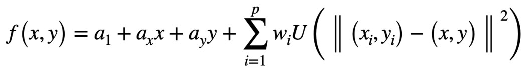
Image with an original grid:

Original space before the TPS transformation.

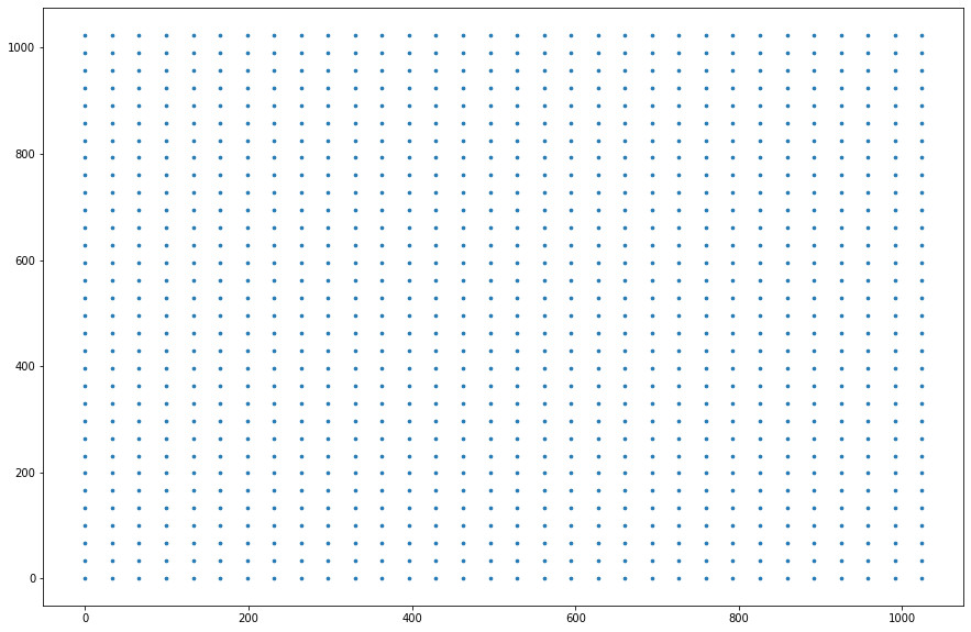
Transformed space after the TPS transformation.

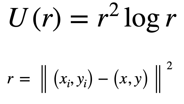
We have the X, Y values and we want the a1, ax, ay and wi values to complete the equation. U is another equation:

To obtain the values that we need we can first represent the problem as a linear system:

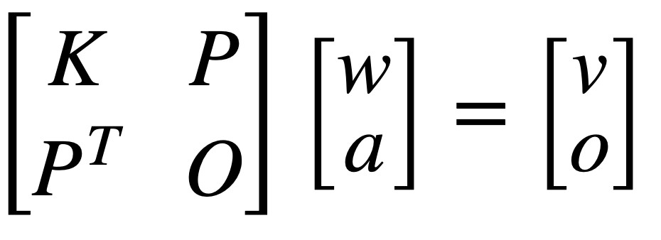
We can notice that this is similar to the TPS equation where if we make a matrix multiplication between the first two terms of the linear system we have that:

w multiplies K

a multiplies P

w multiplies PT

a multiplies O

w contains p w values, K is U(r)

a contains a1, ax, ay, P is (1, xi, yi)

PT is the transpose of P

O is a 3x3 matrix of zeros

Finally o is a 3 x 1 column vector of zeros and v contains v p elements, where v are the target coordinates where each xi and yi are going to end after the transformation.

We obtain the v values by shifting each point in the grid representation of the image by a random distance, thus, we have the coordinates where the image starts (The grid) and the coordinates where we want each point of the image to move (v) so we can learn the transformation that leads to these results and use this transformation to augment our image.

We may realize that we already have all the values except for w and a. Hence in order to solve the equation we have to write the linear sistem in terms of w and a:

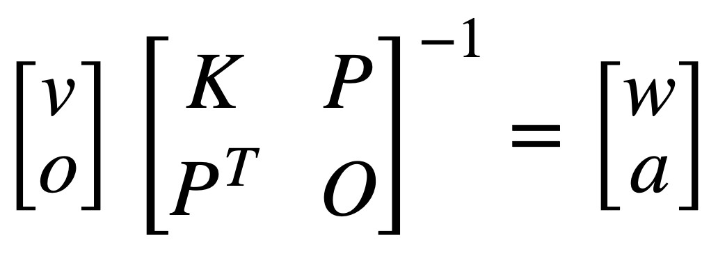
the matrix that contains K, P, PT and O is now on the other side of the equation as its inverse. This matrix is called L and its inverse Li. One thing that is important to mention is that as we have more p control points, the computation of the inverse of L (Li) gets more and more complex. Due to this, we often only use a part of the space as control points and not the whole space so the complexity of the equation is reduced.

Now that we know the TPS equation, let's implement it using python and TensorFlow.

TensorFlow Code

The create_tps function contains the implementation of the TPS equation:

def create_tps(height=256, width=512):

  grid_size = 3

  axis_coords_x = tf.linspace(0, height * 2, grid_size)

  # when default params: ([  0., 256., 512.]), shape 3

  axis_coords_x = tf.cast(axis_coords_x, tf.float32)



  axis_coords_y = tf.linspace(0, width * 2, grid_size)

  # when default params: ([   0.,  512., 1024.]), shape 3

  axis_coords_y = tf.cast(axis_coords_y, tf.float32)



  N = 13

  P_Y, P_X = tf.meshgrid(axis_coords_x, axis_coords_y) # control points

  # Each shape (grid_size, grid_size)



  # when default P_X is

  # [[  0., 256., 512.],

  # [  0., 256., 512.],

  # [  0., 256., 512.]])



  # when default P_Y is

  # [[   0.,    0.,    0.],

  # [ 512.,  512.,  512.],

  # [1024., 1024., 1024.]]



  P_X = tf.reshape(P_X, (-1, 1)) # shape (grid_size * grid_size, 1)

  P_Y = tf.reshape(P_Y, (-1, 1)) # shape (grid_size * grid_size, 1)



  scale = (width * 2) * 0.1

  random_points_x = tf.random.uniform(P_X.shape, minval=-scale, maxval=scale)

  random_points_y = tf.random.uniform(P_Y.shape, minval=-scale, maxval=scale)



  DST_X = P_X + random_points_x

  DST_Y = P_Y + random_points_y

As mentioned earlier, we model the image as a grid (P_X, P_Y) and shift each pixel by a random distance to obtain v (DST_X, DST_Y). We can observe that we are not using a grid of the same size of the image but a smaller one of size 9x9 to reduce the computation time.

  # corners of the grid 0, width * 2  0, height * 2

  corner_points_x = tf.expand_dims([0, 0, width * 2, width * 2], axis=1)

  corner_points_x = tf.cast(corner_points_x, tf.float32)



  corner_points_y = tf.expand_dims([0, height * 2, 0, height * 2], axis=1)

  corner_points_y = tf.cast(corner_points_y, tf.float32)



  DST_X = tf.concat([DST_X, corner_points_x], axis=0) # shape ((grid_size * grid_size) + 3, 1) or (N, 1)

  DST_Y = tf.concat([DST_Y, corner_points_y], axis=0) # shape ((grid_size * grid_size) + 3, 1) or (N, 1)



  Q_X = DST_X

  Q_Y = DST_Y



  Q_X = tf.cast(Q_X, tf.float32) # shape (13, 1)

  Q_Y = tf.cast(Q_Y, tf.float32) # shape (13, 1)

  # contains the modified grid, grid + random points and corner points



  P_X = tf.concat([P_X, corner_points_x], axis=0) # shape (13, 1)

  P_Y = tf.concat([P_Y, corner_points_y], axis=0) # shape (13, 1)

  # contains the original grid and corner points

We add the corners of the grid to the original grid and the final coordinates v, thus making the final grid and v of size (N, N) in this case 13x13. Hence we can say our p is 13 or N. This is done so the corners, [0, height], [0, width] always maps to the same coordinates [0, height], [0, width] and we keep the aspect of the image.

  Li = get_L_inverse(Q_X, Q_Y)  # shape (16, 16)

Li is the same matrix Li in the TPS equation, the code for this function is:

def get_L_inverse(X, Y):

  N = X.shape[0]

  Xmat = tf.repeat(X, repeats=[13], axis=1) # Expand to right 9x9

  Ymat = tf.repeat(Y, repeats=[13], axis=1) # Expand to right 9x9



  P_dist_squared = tf.square(Xmat - tf.transpose(Xmat)) + tf.square(Ymat - tf.transpose(Ymat))

  P_dist_squared = tf.where(tf.equal(P_dist_squared, 0), tf.ones_like(P_dist_squared), P_dist_squared)

  K = P_dist_squared * tf.math.log(P_dist_squared)



  O = tf.ones([N, 1], dtype=tf.float32)

  Z = tf.zeros([3, 3], dtype=tf.float32)

  P = tf.concat([O, X, Y], axis=1)

  L = tf.concat([tf.concat([K, P], axis=1), tf.concat([tf.transpose(P), Z], axis=1)], axis=0)



  Li = tf.linalg.inv(L)



  return Li

Inside this function we build the Li matrix to solve the TPS equation, The names of each variable are a little bit different but represent the same, for instance Z is O, P is the same, O is o. We build k by using the equation U and we transpose X and Y to subtract each pixel xi and yi from the whole grid X, Y in a easier way.

We can notice that to build the Li matrix we use v (Q_X, Q_Y) instead of X, Y (DST_X, DST_Y) so here we change the order and make the target coordinates the original coordinates and the X, Y the target coordinates.

  P_X = tf.expand_dims(P_X, 0) # shape (1, 13, 1)

  P_Y = tf.expand_dims(P_Y, 0) # shape (1, 13, 1)



  Li = tf.expand_dims(Li, 0) # shape (1, 16, 16)



  W_X = tf.linalg.matmul(Li[:, :N, :N], P_X) # Automatic broadcast for Li

  W_Y = tf.linalg.matmul(Li[:, :N, :N], P_Y) # Automatic broadcast for Li

  # 1, 13, 13 * 1, 13, 1

  # Ignoring first dimension 13, 13 * 13, 1 == 13, 1

  # shape (1, 13, 1)



  W_X = tf.expand_dims(W_X, 3)

  W_X = tf.expand_dims(W_X, 4)

  # shape (1, 13, 1, 1, 1)

  W_X = tf.transpose(W_X, [0, 4, 2, 3, 1])

  # shape (1, 1, 1, 1, 13)



  W_Y = tf.expand_dims(W_Y, 3)

  W_Y = tf.expand_dims(W_Y, 4)

  # shape (1, 13, 1, 1, 1)

  W_Y = tf.transpose(W_Y, [0, 4, 2, 3, 1])

  # shape (1, 1, 1, 1, 13)



  # compute weights for the affine part

  A_X = tf.linalg.matmul(Li[:, N:, :N], P_X) # Automatic broadcast for Li

  A_Y = tf.linalg.matmul(Li[:, N:, :N], P_Y) # Automatic broadcast for Li

  # 1, 3, 13 * 1, 13, 1

  # Ignoring first dimension 3, 13 * 13, 1 == 3, 1

  # shape (1, 3, 1)



  A_X = tf.expand_dims(A_X, 3)

  A_X = tf.expand_dims(A_X, 4)

  A_X = tf.transpose(A_X, [0, 4, 2, 3, 1])



  A_Y = tf.expand_dims(A_Y, 3)

  A_Y = tf.expand_dims(A_Y, 4)

  A_Y = tf.transpose(A_Y, [0, 4, 2, 3, 1])

  # shape (1, 1, 1, 1, 3)

To obtain w and a we have to compute the matrix multiplication between Li and [v, o] (or in this case X, Y since we changed the order).

With w and a now we have all the required values to compute the TPS equation:

  grid_Y, grid_X = tf.meshgrid(tf.linspace(0, width * 2, width), tf.linspace(0, height * 2, height)) # 0, 256, 512

  # shape (256, 512)



  grid_X = tf.expand_dims(tf.expand_dims(grid_X, 0), 3)

  grid_Y = tf.expand_dims(tf.expand_dims(grid_Y, 0), 3)

  # shape (1, 256, 512, 1)



  points = tf.concat([grid_X, grid_Y], axis=3)

  points = tf.cast(points, tf.float32)

  # shape (1, 256, 512, 2)



  points_X_for_summation = tf.expand_dims(points[:, :, :, 0], axis=-1) # shape (1, 256, 512, 1)

  points_Y_for_summation = tf.expand_dims(points[:, :, :, 1], axis=-1)

As the first step, we build another grid (points_X_for_summation, points_Y_for_summation) but this time we use the whole image area, so that the grid is not anymore NxN but the same size of the image.

  # change to Q

  Q_X = tf.expand_dims(Q_X, 2)

  Q_X = tf.expand_dims(Q_X, 3)

  Q_X = tf.expand_dims(Q_X, 4)

  Q_X = tf.transpose(Q_X) # shape (1, 1, 1, 1, 13)



  Q_Y = tf.expand_dims(Q_Y, 2)

  Q_Y = tf.expand_dims(Q_Y, 3)

  Q_Y = tf.expand_dims(Q_Y, 4)

  Q_Y = tf.transpose(Q_Y) # shape (1, 1, 1, 1, 13)



  delta_X = Q_X - tf.expand_dims(points_X_for_summation, axis=-1)

  delta_Y = Q_Y - tf.expand_dims(points_Y_for_summation, axis=-1)

  # shape 1, 256, 512, 1, 13

We reshape Q_X and Q_Y in order to subtract them from the complete grid

  dist_squared = tf.square(delta_X) + tf.square(delta_Y)

  dist_squared = tf.where(tf.equal(dist_squared, 0), tf.ones_like(dist_squared), dist_squared) # remove 0 values

  U = dist_squared * tf.math.log(dist_squared)

  # shape 1, 256, 512, 1, 13

Compute U

  points_X_prime = A_X[:, :, :, :, 0] + (A_X[:, :, :, :, 1] * points_X_for_summation) + (A_X[:, :, :, :, 2] * points_Y_for_summation)

  points_X_prime += tf.keras.backend.sum((W_X * U), axis=-1)



  points_Y_prime = A_Y[:, :, :, :, 0] + (A_Y[:, :, :, :, 1] * points_X_for_summation) + (A_Y[:, :, :, :, 2] * points_Y_for_summation)

  points_Y_prime += tf.keras.backend.sum((W_Y * U), axis=-1)

  # shape (1, 256, 512, 1)



  warped_grid = tf.concat([points_X_prime, points_Y_prime], axis=-1)

  # shape (1, 256, 512, 2)



  return warped_grid

Finally we use w and a to compute the TPS equation and transform the complete grid (points_X_for_summation, points_Y_for_summation) from the original normal coordinates to a target random coordinates.

We can notice that in order to compute the w and a values we use a subset of the complete grid (P_X, P_Y) and not the complete pixel space (points_X_for_summation, points_Y_for_summation), this is done to reduce computation time and complexity, thus the computed w and a are just an aproximation of the real w and a values for the complete grid, but an enough one to compute the TPS equation.

If you want to know more about TPS the lecture of the paper Approximate Thin Plate Spline Mappings is a recommendation.

Interpolation

Using the create_tps function we can get a transformed grid space, we can use this transformed space to agument an image of the same size using interpolation:

def tps_augmentation(img, tps, height=256, width=512):

  new_max = width

  new_min = 0

  grid_x = (new_max - new_min) / (tf.keras.backend.max(tps[:, :, :, 1]) - tf.keras.backend.min(tps[:, :, :, 1])) * (tps[:, :, :, 1] - tf.keras.backend.max(tps[:, :, :, 1])) + new_max



  new_max = height

  new_min = 0

  grid_y = (new_max - new_min) / (tf.keras.backend.max(tps[:, :, :, 0]) - tf.keras.backend.min(tps[:, :, :, 0])) * (tps[:, :, :, 0] - tf.keras.backend.max(tps[:, :, :, 0])) + new_max



  grid = tf.stack([grid_x, grid_y], axis=-1)



  final_image = tfa.image.resampler(tf.expand_dims(img, axis=0), grid)



  return final_image[0]

The tfa.image.resampler function takes a normalized grid, between [0, 1], and transforms the given image according to the grid, like the Normal input and label images of the next section.

What makes TPS great for the data augmentation task is the fact that this technique introduces a smooth factor to the equation, in this way, the transformation from the original coordinates to the target coordinates obeys a smooth path, something that could not be achieved using only random target coordinates.

DeepSIM

This paper presents the idea of single image training using TPS as data augmentation. As we know, using little data to train a model only leads to overfitting, even when traditional data augmentation techniques, like rotation, crop or zoom, are used, this is often not enough to bypass the stated problem.

However, with the help of TPS as a data augmentation tool, we can generate images varied enough to overcome the overfitting problem. Therefore, the idea is simple, we augment the pair input, label images with the same TPS augmentation and train the network.

Here we train a conditional GAN which generator uses the pix2pixHD architecture, and along with the adversarial loss, we use the l1 loss and the perceptual loss. The whole framework is easy to implement and also easy to train and shows the potential of TPS for data augmentation.

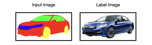
Normal input and label images

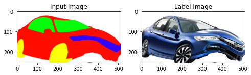
Label and input images after the TPS transformation

Color2Embed

On this occasion, we meet the task of image colorization. In this task, we have two images, a reference color image, and a target grayscale image, and the job is to extract color information from the reference image and inject such information into the target image to achieve colorization.

The challenge here is the selection of the reference color images since these images should match the color features of the target grayscale images. If we use the same image as reference and target inputs, the network could just copy each pixel from the reference image to the target image and learn nothing about color extraction.

Consequently, the problem is to find a reference image with a similar style/color information but different content information. As we have seen, this can be done by using the same image for reference and target inputs but transforming the former using TPS augmentation. Hence, the reference image still contains the necessary color information but with notable transformed content information to constrain the network to learn about color extraction.

This time we have a generator model that takes as input the target grayscale image and a color encoder network based on a pre-trained VGG model that takes as input the reference image to obtain the color information to subsequently inject this information to the target image using weight modulation.