Correlation and causality

This two topics are usually confused, may you have hear that correlation does not imply causality, two variables or features have a correlation if the change in the value of one feature affects the value of the other feature, there is a popular example, in New York the price of a slice of pizza gets more expensive or gets cheaper at the same time that the price of the train, we have a correlation between these two variables but one variable is not the reason why the other gets affected, the inflation is the variable that affects the prices of these two products.

True (Positive, Negative) False (Positive, Negative)

• True Positive (TP): When the model predicts correctly the positive class.

• True Negative (TN): When the model predicts correctly the negative class.

• False Positive (FP): When the model predicts incorrectly the positive class.

• False Negative (FN): When the model predicts incorrectly the negative class.

There is a trick to remember this, the word in the right (Positive, Negative) is the class that the model predicts whereas the word in the left tells if the model is right (True) or not (False)

Accuracy

Now we can define accuracy like the ratio of correctly labeled examples to the whole pool of examples.

Accuracy = Number of correct predictions / total number of predictions

Accuracy = TP + TN / FP + FN + TP + TN

Precision and Recall

Accuracy is a good metric but only when you have a balanced dataset (same number of examples per class), if we have a dataset about tumors and we have 91 examples of the negative class (benign) and 9 examples of the positive class (malignant), if we had a model that predicts all the examples as negatives (benign):

True positives examples (TP): 0

True negative example (TN): 91

False positives examples (FP): 0

False negative examples (FN): 9

Accuracy = 0 + 91 / 0 + 9 + 0 + 91

Accuracy = 91 / 100 = 0.91

We would have an accuracy of 91% with a model that classifies all the examples as negative, we should use a different measure:

Precision

The Precision indicates the ratio of corrected classified examples (what percentage of tumors classified as malignant are really malignant):

Precision = TP / TP + FP

If precision is 1 the model no produces False positives.

If we use this metric with a model with the following predictions:

TP = 1

TN = 90

FP = 1

FN = 8

9 positive examples (malignant class) and 91 negative examples (benign class)

Precision = 1 / 1 + 1

We obtained a precision of 0.5, this means that only the 50% of the examples classified as malignant are correctly labeled.

Recall or sensitivity

Recall indicates the proportion of the true positive examples which are labeled as it.

(What proportion of malignant tumors were labeled as malignant)

Recall = TP / TP + FN

If recall is 1 the model no produces false negatives

Recall = 1 / 1 + 8

We obtained a recall of 0.11, the model only labeled correctly the 11% of the malignant examples, we have 9 positive examples and the model only labeled correctly one example as malignant.

ROC Curve

The ROC Curve compare the true positive rate against the false negatives rate

True positive rate (TPR) = TP / TP + FN (This is the same than Recall)

False positive rate (FPR) = FP / FP + TN

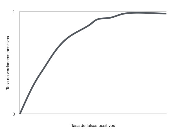
We want this curve to be the most possibly near to the true positive rate.

AUC: Area under the ROC curve

With the area under the ROC curve we can measure the performance of the model

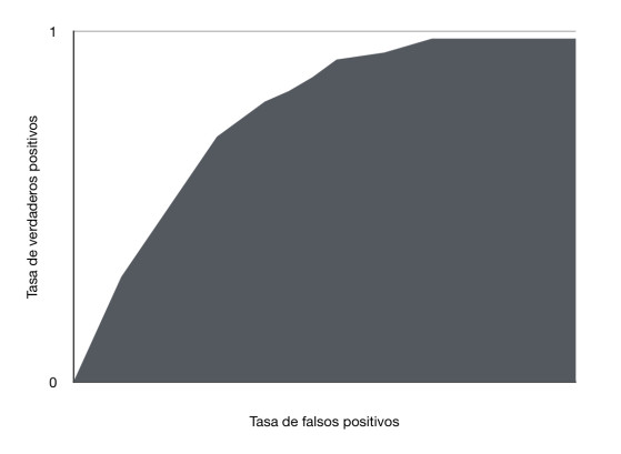
If the area is 1 then the model classified everything correctly, if the area is 0 the model classified the positive examples as negative and the negative examples as positive.

The problem with this metric is that it does not show the false negative rate or true negative rate, with this metric we can optimize the positive class, however if the cost of the false class is higher or we want to optimize the false class we should use a different metric.

Bias-variance Trade Off

We can say that:

• High Bias: Underfitting problem.

High Variance: Overfitting problem.

• Low Bias: No problem.

• Low Variance: No problem.

Lets see 3 examples:

1. We have a margin of error of 1% in the training set and a margin of error of 30% in the validation set, in this case we have high variance due to the fact that the model is performing well in the training set but badly in the validation set (overfitting).

2. We have a margin of error of 40% in the training set and a margin of error of 55% in the validation set, in this case we have high bias in both sets since the model is performing badly in both datasets (Underfitting).

3. We have a margin of error of 0.6% in the training set and a margin of error of 1% in the validation set, in this case we have Low bias since both datasets are performing well and Low variance since we don’t have an (overfitting) problem.

Regularization

We can use regularization to avoid and fix overfitting problems, there are two commonly used algorithms:

L2 (Ridge)

The formula of this algorithm is:

L2 = |W ^ 2|

| | means we obtain the absolute value, if the formula's result is -5 negative the formula will return 5 positive, we need a positive value that adds weigh to the loss function.

In this algorithm if the weights W have big values the model is penalized, as we can remember if W has a big value then the feature related to this weight is more important for the model but we could end up with an overfitting problem where the model only cares about this feature, if we avoid using big values for W the model will have to use more features to obtain the same accuracy.

We also use an hyperparameter called lambda ?, this hyperparameter indicates how strong the regularization is

? * L2

L1 (LASSO)

As we previously saw L2 algorithm want weights values to be small or near to 0, the L1 algorithm wants weights values to be 0.

L1 = |W|

L1 finds the features that are not helpfully for the model and use values of 0 for the weights to cancel these features, we could use this algorithm as feature selection.

Collinearity

The collinearity happens when two independent variables are correlated with each other, this is a problem that affects some models.

Multicollinearity

Multicollinearity happens when one independent variable is correlated with more independent variables. We can resolve this problem using Lasso Regression or Ridge Regression that are regression models with the regularizations L1 or L2*, we can use L1 to cancel the correlated features.

Curse of Dimensionality

This happens when the number of features is very large relative to the number of registers, each feature needs one dimension, if we have 20 features we need 20 dimensions for instance a more complex model.

Dimensionality Reduction

We can use some techniques to remove features from a dataset and fix Curse of Dimensionality problems.

Feature Selection

In Feature Selection as its name suggests we select the features we want to keep, we can use Backward Feature Elimination and Forward Feature Selection techniques.

Feature Extraction

Feature Extraction transform the dataset in order to remove some features. A commonly used algorithm is PCA (Principal Component Analysis).

Ensembles

An ensemble are several models combined to obtain a stronger prediction. Random forest is probability the most famous ensemble, this model uses several decision trees to compute a final prediction, if we have a classification problem the prediction will be the most commonly occurring prediction of the decision trees and for regression problems the prediction will be the mean of the decision trees predictions.

We can use two techniques to build ensembles:

• Bagging:

  • The main objective is reducing the variance and avoid overfitting in order to improve Accuracy.

  • Bagging gives the same weight to all the models no matter if one is better that others.

  • Bagging uses random sampling to train each model, therefore you can train several models in parallel.

  • We can fix overfitting problems with this technique.

• Boosting:

  • The main objective is reducing the bias.

  • Boosting gives more weight to the best models.

  • Boosting trains the models sequentially to improve each model, you can not train these models in parallel.

  • We can fix underfitting problems with this technique.