In this post, I will talk about different techniques that you can try to improve the results of your neural networks. Additionally, we will use a technique called weight pruning to reduce the size of the final model.

To create the neural network we will use TensorFlow 2.0 and tf.Keras.

You can check the complete code of this post in this Jupyter Notebook.

Our Model

We will implement the following model:

def create_vgg_model():

  input = layers.Input(input_img_size)



  model = layers.Conv2D(64, 3, padding='same', activation='relu')(input)

  model = layers.Conv2D(64, 3, padding='same', activation='relu')(model)

  model = layers.MaxPool2D(2, strides=2, padding='same')(model)



  model = layers.Conv2D(128, 3, padding='same', activation='relu')(model)

  model = layers.Conv2D(128, 3, padding='same', activation='relu')(model)

  model = layers.MaxPool2D(2, strides=2, padding='same')(model)



  model = layers.Conv2D(256, 3, padding='same', activation='relu')(model)

  model = layers.Conv2D(256, 3, padding='same', activation='relu')(model)

  model = layers.Conv2D(256, 3, padding='same', activation='relu')(model)

  model = layers.MaxPool2D(2, strides=2, padding='same')(model)



  model = layers.Conv2D(512, 3, padding='same', activation='relu')(model)

  model = layers.Conv2D(512, 3, padding='same', activation='relu')(model)

  model = layers.Conv2D(512, 3, padding='same', activation='relu')(model)

  model = layers.MaxPool2D(2, strides=2, padding='same')(model)



  model = layers.Conv2D(512, 3, padding='same', activation='relu')(model)

  model = layers.Conv2D(512, 3, padding='same', activation='relu')(model)

  model = layers.Conv2D(512, 3, padding='same', activation='relu')(model)



  model = layers.GlobalAveragePooling2D()(model)



  model = layers.Dense(num_classes, activation="softmax", kernel_initializer='uniform')(model)



  model = Model(inputs=input, outputs=model)



  return model

This is a model based on the VGG architecture, modified to output activation maps easily. However, since TensorFlow 2.0 is brand new, I had problems getting the activation maps, therefore, we won't see them. Once TensorFlow improves I will try fixing this.

Cyclical Learning Rates

As we know, the learning rate is the most important hyperparameter to tune in a neural network. Therefore, we will use a technique called Cyclical Learning Rate to vary the learning rate between bounds, the learning rate starts at a minimum value, increases until it reaches a maximum value and decreases to the minimum value. Besides, when the learning rate increases the training is faster. This and the following section are based on this paper called Cyclical Learning Rates for Training Neural Networks.

Due to this learning rate change, we have improvements in the training, for example, saddle points have small gradients that slow the learning process, when the value of the learning rate increases we can escape from these areas easily.

As we can remember, a gradient contains the information about the path we should follow in order to reduce the loss value, specifically it contains the magnitude/size and the direction, a saddle point is a flat area where the magnitude is quite small.

Another advantage is that we don't have to tune the learning rate value anymore and the optimal learning rate value will be between the minimum and maximal value.

Before implementing this technique we have to know some things:

• A complete cycle: Is the process where the learning rate starts at a minimum value, increases to a maximum value and finally decreases to the minimum value.

• Stepsize: is the number of iterations that the learning rate takes to complete half a cycle, in other words, the number of iterations that the learning rate takes to go from the minimum value to the maximum value.

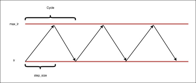
Image from https://github.com/bckenstler/CLR where the original keras implementation is.

A Good value for the stepsize variable is 2 ? 10 times the number of iterations in an epoch, where the number of iterations in an epoch is the size of the dataset between the batch size

In our dataset, we have 5232 images for training and a batch size of 32. Thus, each epoch has 5232/32 iterations. If we use a stepsize value of 4 * iterations a complete cycle will take 8 epochs to complete. Therefore, we should train our neural network for at least 8 epochs to complete a cycle and give the learning rate the opportunity to increase and decrease its value. In fact, it's best to stop training at the end of a complete cycle when the learning rate value is at the minimum value. For example, we should train our neural network for 8, 16, 24, 32 epochs to always complete all the cycles.

Now that we have a background about Cyclical Learning Rates we can code the callback to change the learning rate. Firstly, we need to define the minimum and maximum values that the learning rate will take and the number of epochs:

epochs = 32

min_learning_rate = 1e-3

max_learning_rate = 1e-1

In the following code, we create a new callback:

class CycleLearningRate(tf.keras.callbacks.Callback):

  def __init__(self, model, policy="triangular"):

    super(CycleLearningRate, self).__init__()

    self.model = model

    self.training_iterations = 0

    self.cycle_iterations = 0

    self.history = {}

    self.step_size = 4 * train_steps



    if policy == "triangular":

      self.policy_fn = lambda x: 1.

    else:

      self.policy_fn = lambda x: 1 / (2. ** (x - 1))



  def compute_learning_rate(self):

    cycle = np.floor(1 + self.cycle_iterations / (2 * self.step_size))

    x = np.abs(self.cycle_iterations / self.step_size - 2 * cycle + 1)



    return min_learning_rate + (max_learning_rate - min_learning_rate) * np.maximum(0, (1 - x)) * self.policy_fn(cycle)



  def on_train_begin(self, logs={}):

    if self.cycle_iterations == 0:

      tf.keras.backend.set_value(self.model.optimizer.lr, min_learning_rate)

    else:

      tf.keras.backend.set_value(self.model.optimizer.lr, self.compute_learning_rate())



  def on_batch_end(self, batch, logs=None):

    logs = logs or {}



    self.training_iterations += 1

    self.cycle_iterations += 1



    self.history.setdefault('lr', []).append(tf.keras.backend.get_value(self.model.optimizer.lr))

    self.history.setdefault('iterations', []).append(self.training_iterations)



    for k, v in logs.items():

      self.history.setdefault(k, []).append(v)



    tf.keras.backend.set_value(self.model.optimizer.lr, self.compute_learning_rate())

I will explain this callback by functions:

• on_train_begin: If the training process is beginning the function assigns the minimum value to the learning rate, whereas, if the training process is continuing the function computes and updates the learning rate value.

• on_batch_end: When the model finishes a batch or iteration this function registers the values for the learning rate, number of iterations and cycle iterations. Additionally, this function will call the compute_learning_rate function and update the learning rate value.

• compute_learning_rate: This function computes the new value for the learning rate taking into account the number of iterations and the stepsize to increase or decrease the value.

We can notice that in the constructor of the class we define a policy_fn argument, to vary the learning rate we can use different functions, in this case, I defined two: triangular and triangular2.

triangular: Is the base function where the learning rate varies between the minimum and maximum value.

triangular2: It works similarly to the triangular policy except that the maximum value is cut in half at the end of each cycle. Due to this, we have a learning rate decay behaviour.

exp_range: In a similar way than triangular2, this policy reduces the maximum value at the end of each cycle but by an exponential factor.

normal_model = create_vgg_model()

cycle_lr = CycleLearningRate(normal_model, policy="triangular")

optimizer = SGD(lr=min_learning_rate, momentum=0.9)

normal_model.compile(loss=categorical_focal_loss(), optimizer=optimizer, metrics=['acc'])

trained_model = normal_model.fit_generator(train_generator,

                        epochs=epochs,

                        steps_per_epoch=train_steps,

                        callbacks=[checkpoint, cycle_lr],

                        class_weight={0:1.0, 1:0.33},

                        validation_data=val_generator,

                        validation_steps=val_steps,

                        verbose=1)

With the code above we can train our neural network using a Cyclical Learning Rate. You can notice that the model has a custom loss function called focal loss and a class_weight argument since the dataset we are using to train the network is unbalanced, we will see the importance of this in the last section.

Learning Rate Finder

So far we have seen how we can use a cycle learning rate to improve our models and avoid tunning the learning rate. However, we sill have to choose the values for the minimum and maximum bounds, due to this, in the same paper that I mentioned before, the author mentions that we can use the cycle learning rate with the triangular policy to find the values of these two variables.

The idea is simple, we will use a really small value for the minimum like 1e-10 and a really big value for the maximum like 1e+1. Despite the minimum value is quite small for the network to learn, the learning rate will be increasing, once we notice the loss start to decrease we can use that learning rate value as a minimum, in the same way, the learning rate eventually will reach a value that is quite high for the network to learn and the loss will increase, we can use this learning rate value as a maximum.

The following code to find out the learning rate values is from this tutorial where the author improved the original implementation to make it easier to understand. I changed some things from this code. Therefore, if you want a more complete implementation you should check the tutorial mentioned.

class LearningRateFinder:

  def __init__(self, model):

    self.model = model

    self.steps_per_epoch = train_steps

    self.epochs = 5

    self.start_lr = 1e-10

    self.end_lr = 1e+1



    self.learning_rates_tested = []

    self.losses = []

    self.batch_number = 0

    self.average_loss = 0

    self.best_loss = 1e9

    self.beta = 0.98



    self.batch_updates = self.epochs * self.steps_per_epoch

    self.lr_multiplier = (self.end_lr / self.start_lr) ** (1.0 / self.batch_updates)

    self.stop_factor = 4



  def on_batch_end(self, batch, logs):

    current_lr = tf.keras.backend.get_value(self.model.optimizer.lr)

    self.learning_rates_tested.append(current_lr)



    loss_value = logs["loss"]



    self.batch_number += 1



    self.average_loss = (self.beta * self.average_loss) + ((1 - self.beta) * loss_value)

    smooth_loss = self.average_loss / (1 - (self.beta ** self.batch_number))

    self.losses.append(smooth_loss)



    max_loss_allowed = self.stop_factor * self.best_loss



    if self.batch_number > 1 and smooth_loss > max_loss_allowed:

      self.model.stop_training = True

      return



    if self.batch_number == 1 or smooth_loss < self.best_loss:

      self.best_loss = smooth_loss



    new_lr = current_lr * self.lr_multiplier

    tf.keras.backend.set_value(self.model.optimizer.lr, new_lr)



  def plot_model_results(self):

    selected_learning_rates = self.learning_rates_tested[10:-1]

    selected_losses = self.losses[10:-1]



    plt.plot(selected_learning_rates, selected_losses)

    plt.xscale("log")

    plt.xlabel("Learning Rate")

    plt.ylabel("Loss")

    plt.title("learning rate finder")



  def find_lr(self):

    callback = tf.keras.callbacks.LambdaCallback(on_batch_end=lambda batch, logs:

    self.on_batch_end(batch, logs))



    optimizer = SGD(lr=self.start_lr, momentum=0.9)

    self.model.compile(loss="categorical_crossentropy", optimizer=optimizer, metrics=["accuracy"])



    self.model.fit_generator(train_generator, 

                        steps_per_epoch=self.steps_per_epoch,

                        epochs=self.epochs,

                        verbose=1,

                        callbacks=[callback])



    self.plot_model_results()

test_model = None

test_model = create_vgg_model()

lr_finder = LearningRateFinder(test_model)



lr_finder.find_lr()

With the code above we will train a neural network for 5 epochs increasing the learning rate, we will end up with a plot like the following one:

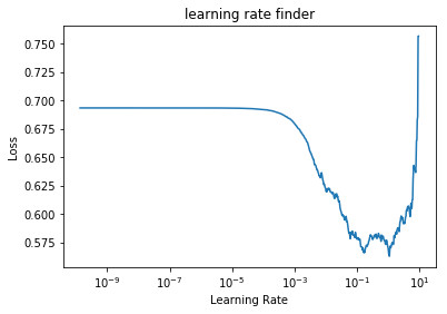
Here we can notice the learning rates values that we should use. when the learning rate value is 1e-3 the loss starts decreasing and when the learning is 1e-1 the loss starts increasing.

If you want to use a learning rate decay you can use the maximum value, in this case 1e-1, and then decrease it epoch by epoch.

Once we have our learning rate values and the model trained we can check the results. In this case, the model reached a validation accuracy of 86%,a sensitivity of 83% and a specificity of 88%. As we can remember our dataset is unbalanced, for this reason, these metrics are quite important

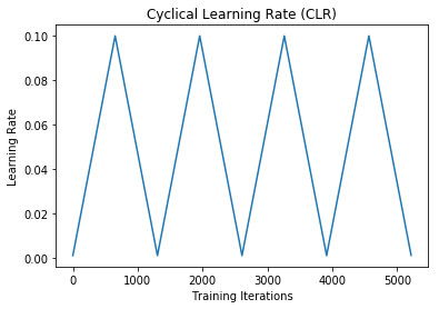
Finally, we can plot how the learning rate values varied:

Weight Pruning

There are several methods to decrease the size of a model, we can make changes to the architecture like reduce the number of kernels or neurons, remove layers, use quantization to use fewer bits to represent the weights. We can also reduce the size of a model by pruning its weights. Thus, we eliminate the unnecessary values in the weight tensor. We achieve this by setting model parameters' values to zero to remove weak connections between layers. We end up with tensors where several values are zero, we call these tensors sparsed tensors. If we compress a model with sparsed tensors we are only keeping the non-zero values.

This section is based on this tutorial from the TensorFlow documentation. However, I will add some useful information that I found like adding cycle learning rate to train the network.

We can implement weight pruning installing the tensorflow-model-optimization package. Once installed, we can choose between prune a model layer by layer or the complete model.

We will start saving our model to compare the size after the pruning:

_, keras_file = tempfile.mkstemp('.h5')

print('model saved: ', keras_file)

tf.keras.models.save_model(normal_model, keras_file, include_optimizer=False)

In order to prune our model we have to train it for more epochs, we have to choose the sparsity value that is the percentage of the weights that are going to be pruned away. Actually, we choose two values, the initial sparsity value and the final sparsity value, we can start with a sparsity of 50% and end up with a value of 90% or start with a value of 0% and end up with 50%, it depends on how much the final size of the model you want it to be and how much accuracy you want to loose. Thus, sparsity is a hyper-parameter that we have to tune.

Another hyper-parameter to tune is the schedule, we have to indicate when the connections will start pruning and how often. For example, if we already have a trained model we can start pruning since the first iteration whereas if we don't have a trained model we should wait to the model to get good accuracy and then start pruning. The frequency value gives the model some time to recover after each pruning step so it can recover some accuracy.

epochs = 8

start_step = 0

end_step = train_steps * epochs



pruning_params = {

      'pruning_schedule': sparsity.PolynomialDecay(initial_sparsity=0.0,

                                                   final_sparsity=0.50,

                                                   begin_step=start_step,

                                                   end_step=end_step,

                                                   frequency=100)

      }

We will train our neural network for 8 epochs, pruning it every 100 iterations starting from a sparsity value of 0% until it reaches a value of 50% and starting in the first iteration.

loaded_model = tf.keras.models.load_model(keras_file)

pruned_model = sparsity.prune_low_magnitude(loaded_model, **pruning_params)



optimizer = SGD(lr=min_learning_rate, momentum=0.9)

pruned_model.compile(loss=categorical_focal_loss(), optimizer=optimizer, metrics=['acc'])

Using the prune_low_magnitude function, we can prune a complete model using the specified hyper-parameters.

cycle_lr = CycleLearningRate(pruned_model, policy="triangular")



pruned_weights_name = "pruned_weight|epoch={epoch:02d}|accuracy={acc:.4f}|val_accuracy={val_acc:.4f}.h5"

checkpoint = ModelCheckpoint(pruned_weights_name, monitor="val_acc", verbose=1, save_weights_only=True, mode="max", save_freq='epoch')



callbacks = [

    sparsity.UpdatePruningStep(),

    cycle_lr,

    checkpoint

]

We just create some callbacks to train or neural network, the sparsity.UpdatePruningStep() function is used to prune the network, here we are saving the weights every epoch so we can use the ones with the best accuracy and sparsity relation. We are also using the CycleLearningRate callback.

The weight pruning technique is based on this paper called [To prune, or not to prune: exploring the efficacy of

pruning for model compression](https://arxiv.org/pdf/1710.01878.pdf)

In this paper, the author mentions that the number of iterations that the model should take to prune the weights and reach the desired sparsity depends on the learning rate. Thus, if we use an excessively small learning rate, the model won't be able to recover from the loss in accuracy caused by the pruned weights. At the same time, if we use a highly big learning rate the weights could be pruned when they have not yet reached good values. The models pruned as an example in the paper used SGD with learning rate decay, weight pruning occurred when the learning rate was still reasonably high to allow the network to recover from the pruned weights.

In the case of cycle learning, the learning rate varies between a minimum and a maximum, we could prune the weights while the learning rate is increasing to allow the network to recover. We can tune a lot of these parameters to achieve the desired sparsity with good accuracy.

Finally, in this pruning process, we obtained different sparsity and accuracy values, we can choose the best option for us, in this case, I chose the weights with 85% of accuracy.

To take advantage of these pruned weights we can compress the whole model to reduce its size. The size of the original model was of 56.19 Mb before compression, after compression, we obtain a size of 51.42 Mb. The size of the pruned model before compression is the same as the original model. If we compress the pruned model, the final size is 38.33 Mb, which is quite good if we take into account that we only lost 1% of accuracy. However, as we can remember our dataset is unbalanced. Due to this, we have to look at more metrics like sensitivity and specificity, the pruned model has a sensitivity of 74% and a specificity of 92%, our specificity increased but our sensitivity decreased and now we could end up with unbalanced predictions. Therefore, we should be careful when pruning models, especially when our dataset is unbalanced.