We have seen several tasks in the field of computer vision like image classification, object detection and gans, in all these tasks we have used convolutional neural networks since this architecture is quite powerful, this time we will see one new task called image segmentation, in this task we have to classify each pixel of some image, for instance the image is divided into multiple segments. There are different ways to achieve this, in this tutorial we will use the U-Net architecture.

Semantic Segmentation

The U-Net architecture takes as input an image like a normal CNN architecture. However, the output of this network is an image typically of the same size as the input image where each pixel is classified to a particular class. The complete name of this task is semantic segmentation, there is another task called instance segmentation where each instance of the class is classified separately like we can see in the following image:

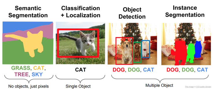
As we can remember in object detection we need the location of each object in the image to compute the loss function and compare the true location with the predicted location, in semantic segmentation we also need the location of the objects, however this time the labels are images, we call these images masks.

We are going to use MRI (Magnetic resonance imaging) images of the brain, some of these brains have tumors, if the brain has a tumor the mask will show it like in the following example:

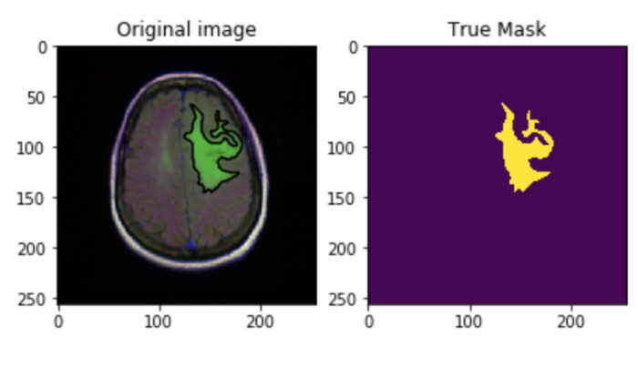
The purple area are just zeros and the yellow area are ones. Therefore, if a pixel is part of the tumor this should be a one. Thanks to this we can use the binary cross entropy loss function to train the neural network.

Network architecture

As I mentioned before the output of our U-Net network is an image, in a normal CNN we have several convolutional layers that extract information from the image and reduce the size of the image until we reach the fully connected layers which compute the classification, we will have a similar behavior except that we don’t have fully connected layers:

def downstream_block(layer, number_filters):

  layer = layers.Conv2D(number_filters, 3, activation='relu', padding="same")(layer)

  cropped_feature_map = layers.Conv2D(number_filters, 3, activation='relu', padding="same")(layer)

  layer = layers.MaxPool2D(2, strides=2, padding='same')(cropped_feature_map)



  return layer, cropped_feature_map

In the code above we have a block that we will repeat 5 times, this block contains two Convolutional Layers and one MaxPool layer

def u_net():

  input = layers.Input(input_shape)

  layer = input



  cropped_feature_maps = []



  for index in range(steps + 1):

    current_number_filters = number_filters * 2 ** index

    layer, cropped_feature_map = downstream_block(layer, current_number_filters)

    cropped_feature_maps.append(cropped_feature_map)



  layer = cropped_feature_maps.pop()

In the code above we defined the input layer which has a input shape of (256, 256, 3) since our images have that size. We repeat the downstream_block five times using each time more filters, finally we use the last cropped_feature_map as our final layer.

You can notice that we save the cropped_feature_map layers since we are going to use them:

def upstream_block(layer, number_filters, cropped_feature_map):

  layer = layers.Conv2DTranspose(number_filters, (2, 2), strides=(2, 2), padding='same')(layer)

  layer = layers.concatenate([layer, cropped_feature_map])

  layer = layers.Conv2D(number_filters, 3, activation='relu', padding="same")(layer)

  layer = layers.Conv2D(number_filters, 3, activation='relu', padding="same")(layer)

Right now our neural network has extracted information from the image, however the size of the last layer is quite small and we need and output of size (256, 256, 1). Therefore, we will apply several transposed convolutions to upsample the input and reach the desire size. In the code above we have a block with two normal convolution layers, one transposed convolution and one concatenate layer, this concatenate layer as its name suggest concatenates two layers, we previously saved some layers from the downstream_block, since we reduce the size of the input image in each convolutional and MaxPool layer we lose some information from the image. In order to fix this we can save some layers which contains important information and concatenate them with the new layers in the upstream_block.

In order to concatenate two layers these must have the same size, sometimes if the input image has a different size we would have to resize one of these layers.

for index in range(steps - 1, -1, -1):

    current_number_filters = number_filters * 2 ** index

    layer = upstream_block(layer, current_number_filters,   cropped_feature_maps[index])



output = layers.Conv2D(1, 1, activation='sigmoid')(layer)

model = Model(input, output)



return model

We run the upstream_block multiple times to upsample the input and finally we use a convolutional layer with the sigmoid activation function to obtain an output image with a minimum value of 0 and a maximum value of 1.

You can download the dataset from Kaggle and see the whole code in this notebook

Results

I trained the neural network with a batch size of 32 and the Adam optimizer for 50 epochs. You can see some predictions below:

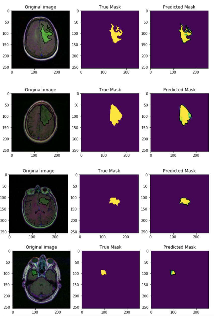
Since the first epoch the accuracy is quite good, almost 100% in the validation set. However, we have to train the neural network for more epochs, 50 is a good number. I also used SGD as optimizer but Adam was a way better even without specify a learning rate.