Oct. 9, 2019
Magnetic resonance imaging and Positron emission tomography Images
This is the second part of two posts where I talk about medical images, you can see the first part in this link. In this post we will see MRI and PET images.
All the code of this post is available in this Jupyter Notebook.
MRI Images
Unlike CT scans, Magnetic resonance imaging scans don't use X-rays. Instead, they use a magnetic field to create images of organs and structures inside your body. Due to this, MRI scans don't produce damaging ionizing radiation like CT scans.
In contrast to CT images, the soft tissue looks better in MRI images and we have a better distinction between grey and white matter.
There is a special kind of MRI called fMRI (Functional magnetic resonance imaging ) which maps brain activity in a similar way that PET scans. However, in this post we will only talk about normal MRI images. We have to know that fMRI images are used in a different way than normal MRI images.
We can find two main types of MRI images, T1 weighted and T2 weighted.
- T1 weighted:
Grey matter is grey, white matter is lighter, fat looks bright, fliuds look dark.
- T2 weighted:
Gray matter is lighter than white matter, fat looks darker, fliuds look bright.
To be sure which type of image we have, we can see the Cerebrospinal fluid CSF which looks white in a T2 weighted image:
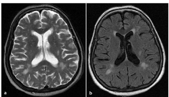
(a) T2 weighted image, (b) T1 weighted image.
NiBabel
In this case we will use the NiBabel library to load the images given that these images have a NIfTI format:
def load_mr_image(file_path):

    image_axis = 2

    medical_image = nib.load(file_path)

    image = medical_image.get_data()

    shape = medical_image.shape


    print(shape)


    image = np.rot90(image)


    image_2d = image[:, :, 144]


    print(image.min(), "Min value")

    print(image.max(), "Max Value")


    plt.style.use('grayscale')

    plt.imshow(image_2d)

    plt.title('Original')

    plt.axis('off')
With the function above we can load and plot a MRI image, additionaly we can print the shape of the image which have 3 dimensions. We can also notice that we rotated the image since the original image has a horizontal orientation.
Improving Images
As well as CT images we can improve the quality of these images, in this case the dataset that I used had a lot of noise which makes this process a little bit different:
def remove_noise_from_image(file_path, slice_num=0, display=False):

    medical_image = nib.load(file_path)

    image = medical_image.get_data()

    shape = medical_image.shape


    image_2d = image[:, :, slice_num]


    image_2d = np.rot90(image_2d)


    # We have to use a number greater than zero since

    # The image contains a lot of noise

    mask = image_2d <= 10


    selem = morphology.disk(2)


    # We have to use the mask to perform segmentation

    # due to the fact that the original image is quite noisy

    segmentation = morphology.dilation(mask, selem)

    labels, label_nb = ndimage.label(segmentation)


    mask = labels == 0


    mask = morphology.dilation(mask, selem)

    mask = ndimage.morphology.binary_fill_holes(mask)

    mask = morphology.dilation(mask, selem)


    clean_image = mask * image_2d


    if display:

        plt.figure(figsize=(15, 2.5))

        plt.subplot(141)

        plt.imshow(image_2d)

        plt.title('Original Image')

        plt.axis('off')


        plt.subplot(142)

        plt.imshow(segmentation)

        plt.title('Background mask')

        plt.axis('off')


        plt.subplot(143)

        plt.imshow(mask)

        plt.title('Brain Mask')

        plt.axis('off')


        plt.subplot(144)

        plt.imshow(clean_image)

        plt.title('Clean Image')

        plt.axis('off')


    return clean_image
In this case first we have to create a mask of the background pixels and from it create the mask of the brain.
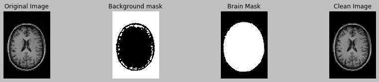

Perhaps it's hard to notice but the second image looks a lot cleaner which could help a deep learning model to recognize the image better.
As aditional information these images have a size of 176x256x256. Therefore, if we get a slice of the axial plane the final 2d image will have a size of 176x256, we can use the add_pad function that we used on the CT images to obtain a image of size 256x256.
Normalization
Unlike CT Images, MRI images don't have a standard scale, the problem with this is the variations caused by the scanner, we can get different intensities from different scanners. Thus, we should apply normalization to fix this problem. Here, I will talk about two great methods, Z-score and Fuzzy C-Means.
Z-score is quite simple, makes the data have zero mean and one unit variance. In this case, we will create a brain mask to only compute the mean and standard deviation from the pixels that belong to the brain area
def standardization(image):

    # Get brain mask

    mask = image == 0


    selem = morphology.disk(2)


    segmentation = morphology.dilation(mask, selem)

    labels, label_nb = ndimage.label(segmentation)


    mask = labels == 0


    mask = morphology.dilation(mask, selem)

    mask = ndimage.morphology.binary_fill_holes(mask)

    mask = morphology.dilation(mask, selem)


    # Normalize


    mean = image[mask].mean()

    std = image[mask].std()


    normalized_image = (image - mean) / std


    return normalized_image
On the other hand, Fuzzy C-Means normalization is more complex. Firstly, we need a mask of the white matter region, we compute the mean only from this area using the mask and finally, normalize the entire image to this mean.
def fcm_normalization(image, norm_value=1):

    white_matter_mask = get_white_matter_mask(image)

    wm_mean = image[white_matter_mask == 1].mean()


    normalized_image = (image / wm_mean) * norm_value


    return normalized_image
You can see the complete functions in the Jupyter Notebook
Fuzzy C-Means is a good choice if we are working with brain images.
If you want to explore more normalization techniques you can look at this repository. From this repository, I get the two methods previously described.
PET Images
Positron emission tomography scans help reveal how the tissues and organs are functioning. These scans use a radioactive drug to show this activity. Commonly, you will see files with names like C-11, F-18 or AV-45 that indicate the type of radioactive tracer/drug used to get the scans. PET scans can be used to evaluate certain brain disorders, such as tumors or Alzheimer's disease.
We will use NiBabel again to load these images:
def load_pet_image(file_path, slice=65):

    medical_image = nib.load(file_path)

    image = medical_image.get_data()

    shape = medical_image.shape


    print(shape)


    image = np.rot90(image)


    image_2d = image[:, :, slice]


    # sum the time axis

    image_2d = np.sum(image_2d, axis=2)


    print(image.min(), "Min value")

    print(image.max(), "Max Value")


    return image_2d
(256, 256, 127, 26)

0.0 Min value

144876.0 Max Value
We can notice that we sum the last axis (2). Since these scans are obtaining to analyze brain functioning through time, we have 4 dimensions, the first three dimensions are the spatial dimensions x, y, z, and the last dimension is the time dimension. Summing this last dimension, we obtain an average PET slice.
Like CT scans, we can apply a lot of the same methods to further preprocess the image, like background remove, resampling to standardize the image and voxel size or just add a pad.
PET images like MRI images don't have a standard scale, in order to compare images from different scanners, intensity normalization should be applied. This normalization can improve our machine learning models as well. We can use the standardization function used in the MRI images to normalize PET images.
Machine learning normalization
To finalize this post I would like to mention that we change the range of these images to train our models since some models with pre-trained weights need a specific range of values. For example, to change the range to [0-1] we can use:
normalized_image = (image - image.min()) / (image.max() - image.min())
To change the range to [0-255]:
normalized_image = (image - image.min()) * (255.0 / (image.max() - image.min()))